# Import all required libraries
import pandas as pd
import numpy as np
import seaborn as sns
import matplotlib.pyplot as plt
from sklearn.decomposition import PCA
from sklearn.manifold import TSNE
from sklearn.preprocessing import StandardScaler
from sklearn.impute import SimpleImputer
import statsmodels.api as sm
import scipy.stats as stats
from scipy.stats import gaussian_kde
from scipy.signal import find_peaks, argrelextrema
from scipy.stats import pearsonr


# Increase font size of all Seaborn plot elements
sns.set(font_scale = 1.25)

# Set Seaborn theme
sns.set_theme(style = "whitegrid")
Data Preprocessing
Lecture 4
Dr. Greg Chism
University of Arizona
INFO 523 - Spring 2024
Warm up
Announcements
RQ 02 is due Wed, Feb 14, 11:59pm
HW 02 is due Wed, Feb 21, 11:59pm
Project 1 proposal reviews will be returned to you by Friday
HW 1 lessons learned
Review HW 1 issues, and show us you reviewed them by closing the issue.
DO NOT hard code local paths!
Instead, you can use {pyprojroot}:
python -m pip install pyprojrootfrom pyprojroot.here import heree.g.,
pd.read_csv(here('data/data.csv'))
Related: data should go into a
datafolder
Narrative/code description text should be plain text under a
###or####header under the appropriate code chunk.
HW 1 lessons learned cont…
- Start early. No late work exceptions will be made in the future
- Ask your peers. I have been monopolized by a few individuals, which is not fair to the rest.
- Peers will likely have the answer
- Peers will likely get to the question before I will.
- Ask descriptive questions. See this page on asking effective questions.
- Please respect my work hours. I will no longer reply to messages after 5pm on work days and at all on weekends.
Setup
Data Preprocessing
Data preprocessing can refer to manipulation, filtration or augmentation of data before it is analyzed, and is often an important step in the data mining process.
Datasets
Human Freedom Index
The Human Freedom Index is a report that attempts to summarize the idea of “freedom” through variables for many countries around the globe.
Environmental Sustainability
Countries are given an overall sustainability score as well as scores in each of several different environmental areas.
Question
How does environmental stability correlate with human freedom indices in different countries, and what trends can be observed over recent years?
Dataset #1: Human Freedom Index
| year | ISO_code | countries | region | pf_rol_procedural | pf_rol_civil | pf_rol_criminal | pf_rol | pf_ss_homicide | pf_ss_disappearances_disap | ... | ef_regulation_business_bribes | ef_regulation_business_licensing | ef_regulation_business_compliance | ef_regulation_business | ef_regulation | ef_score | ef_rank | hf_score | hf_rank | hf_quartile | |
|---|---|---|---|---|---|---|---|---|---|---|---|---|---|---|---|---|---|---|---|---|---|
| 0 | 2016 | ALB | Albania | Eastern Europe | 6.661503 | 4.547244 | 4.666508 | 5.291752 | 8.920429 | 10.0 | ... | 4.050196 | 7.324582 | 7.074366 | 6.705863 | 6.906901 | 7.54 | 34.0 | 7.568140 | 48.0 | 2.0 |
| 1 | 2016 | DZA | Algeria | Middle East & North Africa | NaN | NaN | NaN | 3.819566 | 9.456254 | 10.0 | ... | 3.765515 | 8.523503 | 7.029528 | 5.676956 | 5.268992 | 4.99 | 159.0 | 5.135886 | 155.0 | 4.0 |
| 2 | 2016 | AGO | Angola | Sub-Saharan Africa | NaN | NaN | NaN | 3.451814 | 8.060260 | 5.0 | ... | 1.945540 | 8.096776 | 6.782923 | 4.930271 | 5.518500 | 5.17 | 155.0 | 5.640662 | 142.0 | 4.0 |
| 3 | 2016 | ARG | Argentina | Latin America & the Caribbean | 7.098483 | 5.791960 | 4.343930 | 5.744791 | 7.622974 | 10.0 | ... | 3.260044 | 5.253411 | 6.508295 | 5.535831 | 5.369019 | 4.84 | 160.0 | 6.469848 | 107.0 | 3.0 |
| 4 | 2016 | ARM | Armenia | Caucasus & Central Asia | NaN | NaN | NaN | 5.003205 | 8.808750 | 10.0 | ... | 4.575152 | 9.319612 | 6.491481 | 6.797530 | 7.378069 | 7.57 | 29.0 | 7.241402 | 57.0 | 2.0 |
5 rows × 123 columns
Understand the data
<class 'pandas.core.frame.DataFrame'>
RangeIndex: 1458 entries, 0 to 1457
Data columns (total 123 columns):
 #    Column                              Dtype
---   ------                              -----
 0    year                                int64
 1    ISO_code                            object
 2    countries                           object
 3    region                              object
 4    pf_rol_procedural                   float64
 5    pf_rol_civil                        float64
 6    pf_rol_criminal                     float64
 7    pf_rol                              float64
 8    pf_ss_homicide                      float64
 9    pf_ss_disappearances_disap          float64
 10   pf_ss_disappearances_violent        float64
 11   pf_ss_disappearances_organized      float64
 12   pf_ss_disappearances_fatalities     float64
 13   pf_ss_disappearances_injuries       float64
 14   pf_ss_disappearances                float64
 15   pf_ss_women_fgm                     float64
 16   pf_ss_women_missing                 float64
 17   pf_ss_women_inheritance_widows      float64
 18   pf_ss_women_inheritance_daughters   float64
 19   pf_ss_women_inheritance             float64
 20   pf_ss_women                         float64
 21   pf_ss                               float64
 22   pf_movement_domestic                float64
 23   pf_movement_foreign                 float64
 24   pf_movement_women                   float64
 25   pf_movement                         float64
 26   pf_religion_estop_establish         float64
 27   pf_religion_estop_operate           float64
 28   pf_religion_estop                   float64
 29   pf_religion_harassment              float64
 30   pf_religion_restrictions            float64
 31   pf_religion                         float64
 32   pf_association_association          float64
 33   pf_association_assembly             float64
 34   pf_association_political_establish  float64
 35   pf_association_political_operate    float64
 36   pf_association_political            float64
 37   pf_association_prof_establish       float64
 38   pf_association_prof_operate         float64
 39   pf_association_prof                 float64
 40   pf_association_sport_establish      float64
 41   pf_association_sport_operate        float64
 42   pf_association_sport                float64
 43   pf_association                      float64
 44   pf_expression_killed                float64
 45   pf_expression_jailed                float64
 46   pf_expression_influence             float64
 47   pf_expression_control               float64
 48   pf_expression_cable                 float64
 49   pf_expression_newspapers            float64
 50   pf_expression_internet              float64
 51   pf_expression                       float64
 52   pf_identity_legal                   float64
 53   pf_identity_parental_marriage       float64
 54   pf_identity_parental_divorce        float64
 55   pf_identity_parental                float64
 56   pf_identity_sex_male                float64
 57   pf_identity_sex_female              float64
 58   pf_identity_sex                     float64
 59   pf_identity_divorce                 float64
 60   pf_identity                         float64
 61   pf_score                            float64
 62   pf_rank                             float64
 63   ef_government_consumption           float64
 64   ef_government_transfers             float64
 65   ef_government_enterprises           float64
 66   ef_government_tax_income            float64
 67   ef_government_tax_payroll           float64
 68   ef_government_tax                   float64
 69   ef_government                       float64
 70   ef_legal_judicial                   float64
 71   ef_legal_courts                     float64
 72   ef_legal_protection                 float64
 73   ef_legal_military                   float64
 74   ef_legal_integrity                  float64
 75   ef_legal_enforcement                float64
 76   ef_legal_restrictions               float64
 77   ef_legal_police                     float64
 78   ef_legal_crime                      float64
 79   ef_legal_gender                     float64
 80   ef_legal                            float64
 81   ef_money_growth                     float64
 82   ef_money_sd                         float64
 83   ef_money_inflation                  float64
 84   ef_money_currency                   float64
 85   ef_money                            float64
 86   ef_trade_tariffs_revenue            float64
 87   ef_trade_tariffs_mean               float64
 88   ef_trade_tariffs_sd                 float64
 89   ef_trade_tariffs                    float64
 90   ef_trade_regulatory_nontariff       float64
 91   ef_trade_regulatory_compliance      float64
 92   ef_trade_regulatory                 float64
 93   ef_trade_black                      float64
 94   ef_trade_movement_foreign           float64
 95   ef_trade_movement_capital           float64
 96   ef_trade_movement_visit             float64
 97   ef_trade_movement                   float64
 98   ef_trade                            float64
 99   ef_regulation_credit_ownership      float64
 100  ef_regulation_credit_private        float64
 101  ef_regulation_credit_interest       float64
 102  ef_regulation_credit                float64
 103  ef_regulation_labor_minwage         float64
 104  ef_regulation_labor_firing          float64
 105  ef_regulation_labor_bargain         float64
 106  ef_regulation_labor_hours           float64
 107  ef_regulation_labor_dismissal       float64
 108  ef_regulation_labor_conscription    float64
 109  ef_regulation_labor                 float64
 110  ef_regulation_business_adm          float64
 111  ef_regulation_business_bureaucracy  float64
 112  ef_regulation_business_start        float64
 113  ef_regulation_business_bribes       float64
 114  ef_regulation_business_licensing    float64
 115  ef_regulation_business_compliance   float64
 116  ef_regulation_business              float64
 117  ef_regulation                       float64
 118  ef_score                            float64
 119  ef_rank                             float64
 120  hf_score                            float64
 121  hf_rank                             float64
 122  hf_quartile                         float64
dtypes: float64(119), int64(1), object(3)
memory usage: 1.4+ MB| year | pf_rol_procedural | pf_rol_civil | pf_rol_criminal | pf_rol | pf_ss_homicide | pf_ss_disappearances_disap | pf_ss_disappearances_violent | pf_ss_disappearances_organized | pf_ss_disappearances_fatalities | ... | ef_regulation_business_bribes | ef_regulation_business_licensing | ef_regulation_business_compliance | ef_regulation_business | ef_regulation | ef_score | ef_rank | hf_score | hf_rank | hf_quartile | |
|---|---|---|---|---|---|---|---|---|---|---|---|---|---|---|---|---|---|---|---|---|---|
| count | 1458.000000 | 880.000000 | 880.000000 | 880.000000 | 1378.000000 | 1378.000000 | 1369.000000 | 1378.000000 | 1279.000000 | 1378.000000 | ... | 1283.000000 | 1357.000000 | 1368.000000 | 1374.000000 | 1378.000000 | 1378.000000 | 1378.000000 | 1378.000000 | 1378.000000 | 1378.000000 |
| mean | 2012.000000 | 5.589355 | 5.474770 | 5.044070 | 5.309641 | 7.412980 | 8.341855 | 9.519458 | 6.772869 | 9.584972 | ... | 4.886192 | 7.698494 | 6.981858 | 6.317668 | 7.019782 | 6.785610 | 76.973149 | 6.993444 | 77.007983 | 2.490566 |
| std | 2.582875 | 2.080957 | 1.428494 | 1.724886 | 1.529310 | 2.832947 | 3.225902 | 1.744673 | 2.768983 | 1.559826 | ... | 1.889168 | 1.728507 | 1.979200 | 1.230988 | 1.027625 | 0.883601 | 44.540142 | 1.025811 | 44.506549 | 1.119698 |
| min | 2008.000000 | 0.000000 | 0.000000 | 0.000000 | 0.000000 | 0.000000 | 0.000000 | 0.000000 | 0.000000 | 0.000000 | ... | 0.000000 | 0.000000 | 0.000000 | 2.009841 | 2.483540 | 2.880000 | 1.000000 | 3.765827 | 1.000000 | 1.000000 |
| 25% | 2010.000000 | 4.133333 | 4.549550 | 3.789724 | 4.131746 | 6.386978 | 10.000000 | 10.000000 | 5.000000 | 9.942607 | ... | 3.433786 | 6.874687 | 6.368178 | 5.591851 | 6.429498 | 6.250000 | 38.000000 | 6.336685 | 39.000000 | 1.000000 |
| 50% | 2012.000000 | 5.300000 | 5.300000 | 4.575189 | 4.910797 | 8.638278 | 10.000000 | 10.000000 | 7.500000 | 10.000000 | ... | 4.418371 | 8.074161 | 7.466692 | 6.265234 | 7.082075 | 6.900000 | 77.000000 | 6.923840 | 76.000000 | 2.000000 |
| 75% | 2014.000000 | 7.389499 | 6.410975 | 6.400000 | 6.513178 | 9.454402 | 10.000000 | 10.000000 | 10.000000 | 10.000000 | ... | 6.227978 | 8.991882 | 8.209310 | 7.139718 | 7.720955 | 7.410000 | 115.000000 | 7.894660 | 115.000000 | 3.000000 |
| max | 2016.000000 | 9.700000 | 8.773533 | 8.719848 | 8.723094 | 9.926568 | 10.000000 | 10.000000 | 10.000000 | 10.000000 | ... | 9.623811 | 9.999638 | 9.865488 | 9.272600 | 9.439828 | 9.190000 | 162.000000 | 9.126313 | 162.000000 | 4.000000 |
8 rows × 120 columns
Identifying missing values
year                   0
ISO_code               0
countries              0
region                 0
pf_rol_procedural    578
                    ...
ef_score              80
ef_rank               80
hf_score              80
hf_rank               80
hf_quartile           80
Length: 123, dtype: int64
A lot of missing values 🙃
Data Cleaning
Handling missing data
Options
- Do nothing…
- Remove them
- Imputate
We will be using pf_score from hsi: 80 missing values
Imputation
In statistics, imputation is the process of replacing missing data with substituted values.
Considerations
- Data distribution
- Impact on analysis
- Missing data mechanism
- Multiple imputation
- Can also be used on outliers
Mean imputation
How it Works: Replace missing values with the arithmetic mean of the non-missing values in the same variable.
Pros:
- Easy and fast.
- Works well with small numerical datasets
Cons:
- It only works on the column level.
- Will give poor results on encoded categorical features.
- Not very accurate.
- Doesn’t account for the uncertainty in the imputations.
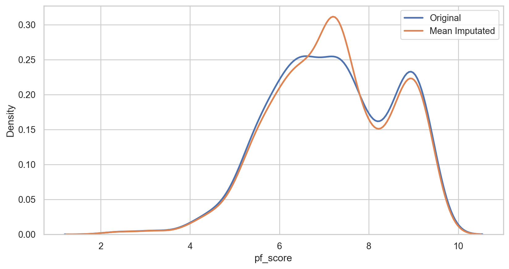
hfi_copy = hfi

mean_imputer = SimpleImputer(strategy = 'mean')
hfi_copy['mean_pf_score'] = mean_imputer.fit_transform(hfi_copy[['pf_score']])

mean_plot = sns.kdeplot(data = hfi_copy, x = 'pf_score', linewidth = 2, label = "Original")

mean_plot = sns.kdeplot(data = hfi_copy, x = 'mean_pf_score', linewidth = 2, label = "Mean Imputated")

plt.legend()

plt.show()hfi_copy = hfi

mean_imputer = SimpleImputer(strategy = 'mean')
hfi_copy['mean_pf_score'] = mean_imputer.fit_transform(hfi_copy[['pf_score']])

mean_plot = sns.kdeplot(data = hfi_copy, x = 'pf_score', linewidth = 2, label = "Original")

mean_plot = sns.kdeplot(data = hfi_copy, x = 'mean_pf_score', linewidth = 2, label = "Mean Imputated")

plt.legend()

plt.show()
Median imputation
How it Works: Replace missing values with the median of the non-missing values in the same variable.
Pros (same as mean):
- Easy and fast.
- Works well with small numerical datasets
Cons (same as mean):
- It only works on the column level.
- Will give poor results on encoded categorical features.
- Not very accurate.
- Doesn’t account for the uncertainty in the imputations.
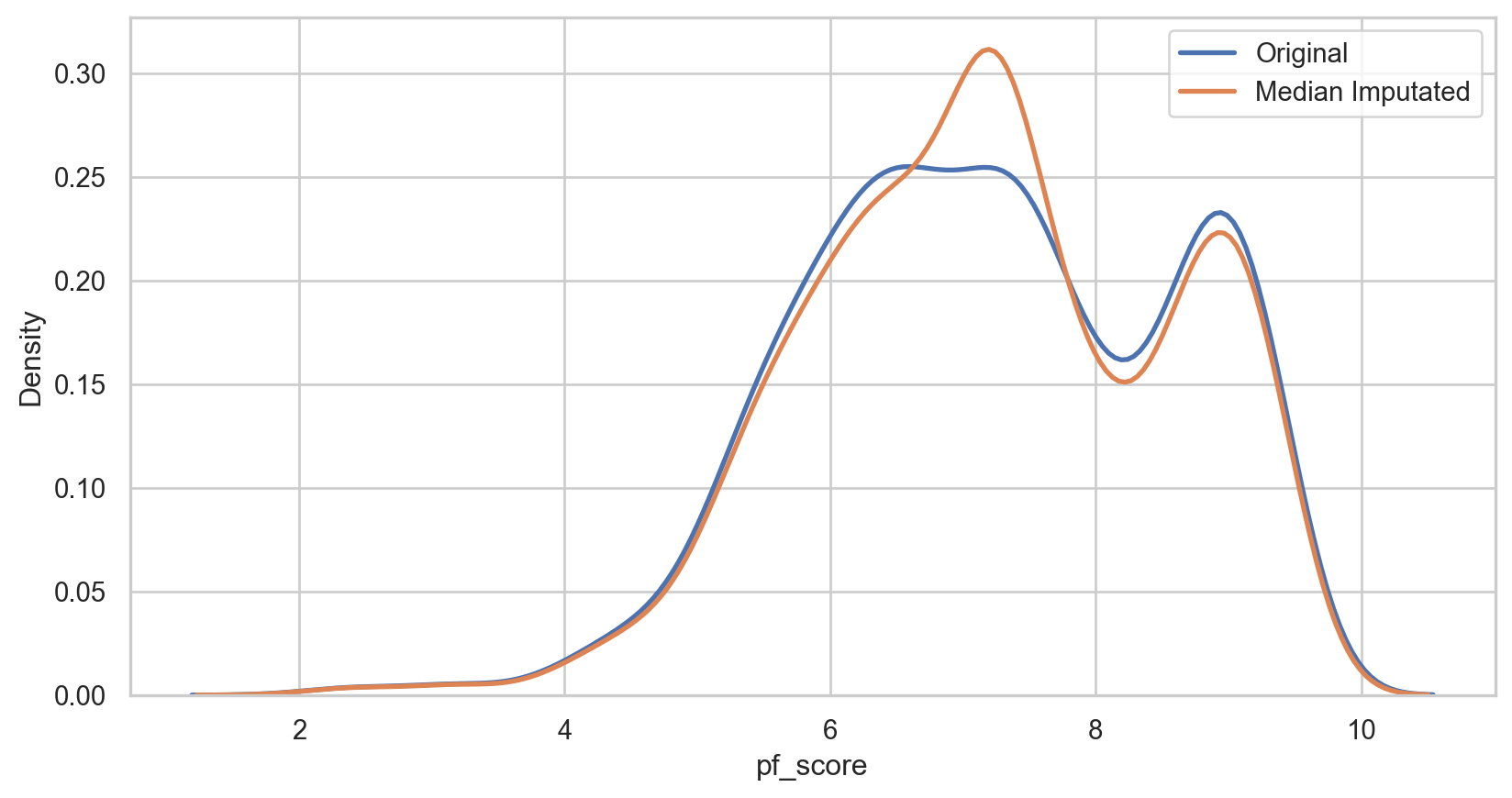
median_imputer = SimpleImputer(strategy = 'median')
hfi_copy['median_pf_score'] = median_imputer.fit_transform(hfi_copy[['pf_score']])

median_plot = sns.kdeplot(data = hfi_copy, x = 'pf_score', linewidth = 2, label = "Original")

median_plot = sns.kdeplot(data = hfi_copy, x = 'median_pf_score', linewidth = 2, label = "Median Imputated")

plt.legend()

plt.show()median_imputer = SimpleImputer(strategy = 'median')
hfi_copy['median_pf_score'] = median_imputer.fit_transform(hfi_copy[['pf_score']])

median_plot = sns.kdeplot(data = hfi_copy, x = 'pf_score', linewidth = 2, label = "Original")

median_plot = sns.kdeplot(data = hfi_copy, x = 'median_pf_score', linewidth = 2, label = "Median Imputated")

plt.legend()

plt.show()
Mode imputation
How it Works: Replace missing values with the mode of the non-missing values in the same variable.
Pros:
- Easy and fast.
- Works well with categorical features.
Cons:
- It also doesn’t factor the correlations between features.
- It can introduce bias in the data.
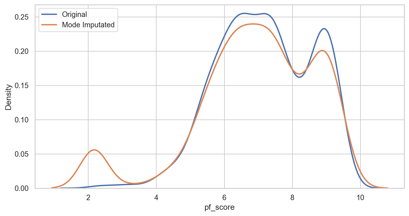
mode_imputer = SimpleImputer(strategy = 'most_frequent')
hfi_copy['mode_pf_score'] = mode_imputer.fit_transform(hfi_copy[['pf_score']])

mode_plot = sns.kdeplot(data = hfi_copy, x = 'pf_score', linewidth = 2, label = "Original")

mode_plot = sns.kdeplot(data = hfi_copy, x = 'mode_pf_score', linewidth = 2, label = "Mode Imputated")

plt.legend()

plt.show()mode_imputer = SimpleImputer(strategy = 'most_frequent')
hfi_copy['mode_pf_score'] = mode_imputer.fit_transform(hfi_copy[['pf_score']])

mode_plot = sns.kdeplot(data = hfi_copy, x = 'pf_score', linewidth = 2, label = "Original")

mode_plot = sns.kdeplot(data = hfi_copy, x = 'mode_pf_score', linewidth = 2, label = "Mode Imputated")

plt.legend()

plt.show()
Capping (Winsorizing) imputation
How it Works: Removing extreme values, or outliers based on cut-offs
Pros:
- Not influenced by extreme values
Cons:
- Capping only modifies the smallest and largest values slightly.
- If no extreme outliers are present, Winsorization may be unnecessary.

upper_limit = np.percentile(hfi_copy['pf_score'].dropna(), 95)
lower_limit = np.percentile(hfi_copy['pf_score'].dropna(), 5)

hfi_copy['capped_pf_score'] = np.clip(hfi_copy['pf_score'], lower_limit, upper_limit)

cap_plot = sns.kdeplot(data = hfi_copy, x = 'pf_score', linewidth = 2, label = "Original")

cap_plot = sns.kdeplot(data = hfi_copy, x = 'capped_pf_score', linewidth = 2, label = "Mode Imputated")

plt.legend()

plt.show()upper_limit = np.percentile(hfi_copy['pf_score'].dropna(), 95)
lower_limit = np.percentile(hfi_copy['pf_score'].dropna(), 5)

hfi_copy['capped_pf_score'] = np.clip(hfi_copy['pf_score'], lower_limit, upper_limit)

cap_plot = sns.kdeplot(data = hfi_copy, x = 'pf_score', linewidth = 2, label = "Original")

cap_plot = sns.kdeplot(data = hfi_copy, x = 'capped_pf_score', linewidth = 2, label = "Mode Imputated")

plt.legend()

plt.show()
Other Imputation Methods
Data type conversion
| year | ISO_code | countries | region | pf_rol_procedural | pf_rol_civil | pf_rol_criminal | pf_rol | pf_ss_homicide | pf_ss_disappearances_disap | ... | ef_regulation | ef_score | ef_rank | hf_score | hf_rank | hf_quartile | mean_pf_score | median_pf_score | mode_pf_score | capped_pf_score | |
|---|---|---|---|---|---|---|---|---|---|---|---|---|---|---|---|---|---|---|---|---|---|
| 0 | 2016-01-01 | ALB | Albania | Eastern Europe | 6.661503 | 4.547244 | 4.666508 | 5.291752 | 8.920429 | 10.0 | ... | 6.906901 | 7.54 | 34.0 | 7.56814 | 48.0 | 2.0 | 7.596281 | 7.596281 | 7.596281 | 7.596281 |
1 rows × 127 columns
Removing duplicates
<class 'pandas.core.frame.DataFrame'>
RangeIndex: 1458 entries, 0 to 1457
Columns: 127 entries, year to capped_pf_score
dtypes: datetime64[ns](1), float64(123), object(3)
memory usage: 1.4+ MB<class 'pandas.core.frame.DataFrame'>
RangeIndex: 1458 entries, 0 to 1457
Columns: 127 entries, year to capped_pf_score
dtypes: datetime64[ns](1), float64(123), object(3)
memory usage: 1.4+ MBNo duplicates! 😊
Filtering data
Let’s look at USA, India, Canada, China
options = ['United States', 'India', 'Canada', 'China']

filtered_hfi = hfi[hfi['countries'].isin(options)]

unique_countries = filtered_hfi['countries'].unique()
print(unique_countries)options = ['United States', 'India', 'Canada', 'China']

filtered_hfi = hfi[hfi['countries'].isin(options)]

unique_countries = filtered_hfi['countries'].unique()
print(unique_countries)options = ['United States', 'India', 'Canada', 'China']

filtered_hfi = hfi[hfi['countries'].isin(options)]

unique_countries = filtered_hfi['countries'].unique()
print(unique_countries)options = ['United States', 'India', 'Canada', 'China']

filtered_hfi = hfi[hfi['countries'].isin(options)]

unique_countries = filtered_hfi['countries'].unique()
print(unique_countries)
['Canada' 'China' 'India' 'United States']Let’s look at Economic Freedom > 75
Transformations
Normalizing
Mean: 5
Standard Deviation: 2
hfi_copy = hfi

scaler = StandardScaler()
hfi_copy[['ef_score_scale', 'pf_score_scale']] = scaler.fit_transform(hfi_copy[['ef_score', 'pf_score']])

hfi_copy[['ef_score_scale', 'pf_score_scale']].describe()hfi_copy = hfi

scaler = StandardScaler()
hfi_copy[['ef_score_scale', 'pf_score_scale']] = scaler.fit_transform(hfi_copy[['ef_score', 'pf_score']])

hfi_copy[['ef_score_scale', 'pf_score_scale']].describe()hfi_copy = hfi

scaler = StandardScaler()
hfi_copy[['ef_score_scale', 'pf_score_scale']] = scaler.fit_transform(hfi_copy[['ef_score', 'pf_score']])

hfi_copy[['ef_score_scale', 'pf_score_scale']].describe()
| ef_score_scale | pf_score_scale | |
|---|---|---|
| count | 1.378000e+03 | 1.378000e+03 |
| mean | 4.524683e-16 | 2.062533e-17 |
| std | 1.000363e+00 | 1.000363e+00 |
| min | -4.421711e+00 | -3.663087e+00 |
| 25% | -6.063870e-01 | -7.303950e-01 |
| 50% | 1.295064e-01 | -8.926277e-03 |
| 75% | 7.068997e-01 | 9.081441e-01 |
| max | 2.722116e+00 | 1.722056e+00 |
Normality test: Q-Q plot
Code
hfi_clean = hfi_copy.dropna(subset = ['pf_score'])

sns.set_style("white")

fig, (ax1, ax2) = plt.subplots(ncols = 2, nrows = 1)

sns.kdeplot(data = hfi_clean, x = "pf_score", linewidth = 5, ax = ax1)
ax1.set_title('Personal Freedom Score')

sm.qqplot(hfi_clean['pf_score'], line = 's', ax = ax2, dist = stats.norm, fit = True)
ax2.set_title('Personal Freedom Score Q-Q plot')

plt.tight_layout()
plt.show()
There were some issues in our plots:
Left Tail: Points deviate downwards from the line, indicating more extreme low values than a normal distribution (negative skewness).
Central Section: Points align closely with the line, suggesting the central data is similar to a normal distribution.
Right Tail: Points curve upwards, showing potential for extreme high values (positive skewness).
Correcting skew
Square-root transformation. √x Used for moderately right-skew (positive skew)
- Cannot handle negative values (but can handle zeros)
Log transformation. log(x+1) Used for substantial right-skew (positive skew)
- Cannot handle negative or zero values
Inverse transformation. 1x Used for severe right-skew (positive skew)
- Cannot handle negative or zero values
Squared transformation. x2 Used for moderately left-skew (negative skew)
- Effective when lower values are densely packed together
Cubed transformation. x3 Used for severely left-skew (negative skew)
- Further stretches the tail of the distribution
Comparing transformations

Moderate negative skew, no zeros or negative values
Code
hfi_clean['pf_score_sqrt'] = np.sqrt(hfi_clean['pf_score'])

col = hfi_clean['pf_score_sqrt']

fig, (ax1, ax2) = plt.subplots(ncols = 2, nrows = 1)

sns.kdeplot(col, linewidth = 5, ax = ax1)
ax1.set_title('Square-root Density plot')

sm.qqplot(col, line = 's', ax = ax2)
ax2.set_title('Square-root Q-Q plot')
plt.tight_layout()
plt.show()hfi_clean['pf_score_sqrt'] = np.sqrt(hfi_clean['pf_score'])

col = hfi_clean['pf_score_sqrt']

fig, (ax1, ax2) = plt.subplots(ncols = 2, nrows = 1)

sns.kdeplot(col, linewidth = 5, ax = ax1)
ax1.set_title('Square-root Density plot')

sm.qqplot(col, line = 's', ax = ax2)
ax2.set_title('Square-root Q-Q plot')
plt.tight_layout()
plt.show()

Code
hfi_clean['pf_score_log'] = np.log(hfi_clean['pf_score'] + 1)

col = hfi_clean['pf_score_log']

fig, (ax1, ax2) = plt.subplots(ncols = 2, nrows = 1)

sns.kdeplot(col, linewidth = 5, ax = ax1)
ax1.set_title('Log Density plot')

sm.qqplot(col, line = 's', ax = ax2)
ax2.set_title('Log Q-Q plot')
plt.tight_layout()
plt.show()hfi_clean['pf_score_log'] = np.log(hfi_clean['pf_score'] + 1)

col = hfi_clean['pf_score_log']

fig, (ax1, ax2) = plt.subplots(ncols = 2, nrows = 1)

sns.kdeplot(col, linewidth = 5, ax = ax1)
ax1.set_title('Log Density plot')

sm.qqplot(col, line = 's', ax = ax2)
ax2.set_title('Log Q-Q plot')
plt.tight_layout()
plt.show()

Code
hfi_clean['pf_score_inv'] = 1/hfi_clean.pf_score

col = hfi_clean['pf_score_inv']

fig, (ax1, ax2) = plt.subplots(ncols = 2, nrows = 1)

sns.kdeplot(col, linewidth = 5, ax = ax1)
ax1.set_title('Inverse Density plot')

sm.qqplot(col, line = 's', ax = ax2)
ax2.set_title('Inverse Q-Q plot')
plt.tight_layout()
plt.show()hfi_clean['pf_score_inv'] = 1/hfi_clean.pf_score

col = hfi_clean['pf_score_inv']

fig, (ax1, ax2) = plt.subplots(ncols = 2, nrows = 1)

sns.kdeplot(col, linewidth = 5, ax = ax1)
ax1.set_title('Inverse Density plot')

sm.qqplot(col, line = 's', ax = ax2)
ax2.set_title('Inverse Q-Q plot')
plt.tight_layout()
plt.show()

Code
hfi_clean['pf_score_square'] = pow(hfi_clean.pf_score, 2)

col = hfi_clean['pf_score_square']

fig, (ax1, ax2) = plt.subplots(ncols = 2, nrows = 1)

sns.kdeplot(col, linewidth = 5, ax = ax1)
ax1.set_title('Squared Density plot')

sm.qqplot(col, line = 's', ax = ax2)
ax2.set_title('Squared Q-Q plot')
plt.tight_layout()
plt.show()hfi_clean['pf_score_square'] = pow(hfi_clean.pf_score, 2)

col = hfi_clean['pf_score_square']

fig, (ax1, ax2) = plt.subplots(ncols = 2, nrows = 1)

sns.kdeplot(col, linewidth = 5, ax = ax1)
ax1.set_title('Squared Density plot')

sm.qqplot(col, line = 's', ax = ax2)
ax2.set_title('Squared Q-Q plot')
plt.tight_layout()
plt.show()

Code
hfi_clean['pf_score_cube'] = pow(hfi_clean.pf_score, 3)

col = hfi_clean['pf_score_cube']

fig, (ax1, ax2) = plt.subplots(ncols = 2, nrows = 1)

sns.kdeplot(col, linewidth = 5, ax = ax1)
ax1.set_title('Cubed Density plot')

sm.qqplot(col, line = 's', ax = ax2)
ax2.set_title('Cubed Q-Q plot')
plt.tight_layout()
plt.show()hfi_clean['pf_score_cube'] = pow(hfi_clean.pf_score, 3)

col = hfi_clean['pf_score_cube']

fig, (ax1, ax2) = plt.subplots(ncols = 2, nrows = 1)

sns.kdeplot(col, linewidth = 5, ax = ax1)
ax1.set_title('Cubed Density plot')

sm.qqplot(col, line = 's', ax = ax2)
ax2.set_title('Cubed Q-Q plot')
plt.tight_layout()
plt.show()

What did we learn?
Negative skew excluded all but Squared and Cubed transformations
Squared transformation was the best
The data is bimodal, so no transformation is perfect
Dealing with multimodality
K-Means Clustering
- We will learn this later
Gaussian Mixture Models
- Also later
Thresholding
- No obvious valley
Domain knowledge
- None that is applicable
Kernel Density Estimation (KDE)
Finding valleys in multimodal data, then splitting
ˆf(x)=1nhn∑i=1K(x−xih)
ˆf(x) is the estimated probability density function at point x.
n is the number of data points.
xi are the observed data points.
h is the bandwidth.
K is the kernel function, which is a non-negative function that integrates to one and is symmetric around zero.
The choice of h and K can significantly affect the resulting estimate.
Common choices for the kernel function K include the Gaussian kernel and Epanechnikov kernel
KDE: bandwidth method
In density estimations, there is a smoothing parameter
Scott’s Rule
- Rule of thumb for choosing kernal bandwidth
- Proportional to the standard deviation of the data and inversely proportional to the cube root of the sample size (n).
- Formula: h=σ⋅n−13
- Tends to produce a smoother density estimation
- Suitable for data that is roughly normally distributed
Silverman’s Rule
- Another popular rule of thumb
- Similar to Scott’s rule but potentially leading to a smaller bandwidth.
- Formula: h=(4ˆσ53n)15
- Can be better for data with outliers or heavy tails
KDE: our data
Code
values = hfi_clean['pf_score_square']
kde = gaussian_kde(values, bw_method = 'scott')
x_eval = np.linspace(values.min(), values.max(), num = 500)
kde_values = kde(x_eval)

minima_indices = argrelextrema(kde_values, np.less)[0]
valleys = x_eval[minima_indices]

plt.figure(figsize = (7, 5))
plt.title('KDE and Valleys')
sns.lineplot(x = x_eval, y = kde_values, label = 'KDE')
plt.scatter(x = valleys, y = kde(valleys), color = 'r', zorder = 5, label = 'Valleys')
plt.legend()
plt.show()

print("Valley x-values:", valleys)values = hfi_clean['pf_score_square']
kde = gaussian_kde(values, bw_method = 'scott')
x_eval = np.linspace(values.min(), values.max(), num = 500)
kde_values = kde(x_eval)

minima_indices = argrelextrema(kde_values, np.less)[0]
valleys = x_eval[minima_indices]

plt.figure(figsize = (7, 5))
plt.title('KDE and Valleys')
sns.lineplot(x = x_eval, y = kde_values, label = 'KDE')
plt.scatter(x = valleys, y = kde(valleys), color = 'r', zorder = 5, label = 'Valleys')
plt.legend()
plt.show()

print("Valley x-values:", valleys)

Valley x-values: [68.39968248]Split the data
valley = 68.39968248
hfi_clean['group'] = np.where(hfi_clean['pf_score_square'] < valley, 'group1', 'group2')

data = hfi_clean[['group', 'pf_score_square']].sort_values(by = 'pf_score_square')
data.head()valley = 68.39968248
hfi_clean['group'] = np.where(hfi_clean['pf_score_square'] < valley, 'group1', 'group2')

data = hfi_clean[['group', 'pf_score_square']].sort_values(by = 'pf_score_square')
data.head()valley = 68.39968248
hfi_clean['group'] = np.where(hfi_clean['pf_score_square'] < valley, 'group1', 'group2')

data = hfi_clean[['group', 'pf_score_square']].sort_values(by = 'pf_score_square')
data.head()
| group | pf_score_square | |
|---|---|---|
| 159 | group1 | 4.693962 |
| 321 | group1 | 5.461029 |
| 141 | group1 | 6.308405 |
| 483 | group1 | 6.345709 |
| 303 | group1 | 8.189057 |
Plot the grouped data

Dimensional reduction
Dimension reduction, is the transformation of data from a high-dimensional space into a low-dimensional space so that the low-dimensional representation retains some meaningful properties of the original data, ideally close to its intrinsic dimension.
Principal component analysis (PCA) - Unsupervised
Maximizes variance in the dataset.
Finds orthogonal principal components.
Useful for feature extraction and data visualization.
t-Distributed Stochastic Neighbor Embedding (t-SNE) - Unsupervised
Preserves local structures and relationships
Maximizes the ratio of between-class variance to within-class variance.
Stochastic and iterative process (probabilistic), iteratively minimizing the divergence between distributions
Ideal for complex data visualization
Dimensional reduction: applied
numeric_cols = hfi.select_dtypes(include = [np.number]).columns

# Applying mean imputation only to numeric columns
hfi[numeric_cols] = hfi[numeric_cols].fillna(hfi[numeric_cols].mean())

features = ['pf_rol_procedural', 'pf_rol_civil', 'pf_rol_criminal', 'pf_rol', 'hf_score', 'hf_rank', 'hf_quartile']

x = hfi.loc[:, features].values
y = hfi.loc[:, 'region'].values
x = StandardScaler().fit_transform(x)
Code
pca = PCA(n_components = 2)
principalComponents = pca.fit_transform(x)
principalDf = pd.DataFrame(data = principalComponents, columns = ['principal component 1', 'principal component 2'])
pca_variance_explained = pca.explained_variance_ratio_
print("Variance explained:", pca_variance_explained, "\n", principalDf)pca = PCA(n_components = 2)
principalComponents = pca.fit_transform(x)
principalDf = pd.DataFrame(data = principalComponents, columns = ['principal component 1', 'principal component 2'])
pca_variance_explained = pca.explained_variance_ratio_
print("Variance explained:", pca_variance_explained, "\n", principalDf)
Variance explained: [0.76138995 0.15849799]
       principal component 1  principal component 2
0             -5.164625e-01           9.665680e-01
1              2.366765e+00          -1.957381e+00
2              2.147729e+00          -1.664483e+00
3              2.784437e-01          -8.066415e-01
4             -3.716205e-01           4.294282e-01
...                     ...                    ...
1453           4.181375e+00           4.496988e-01
1454           5.213024e-01          -6.010449e-01
1455          -1.374342e-16           2.907121e-16
1456           1.545577e+00           5.422255e-01
1457           3.669011e+00          -4.294948e-01

[1458 rows x 2 columns]
Code
# Combining the scatterplot of principal components with the scree plot using the correct column names
fig, axes = plt.subplots(nrows = 1, ncols = 2, figsize = (12, 5))

# Scatterplot of Principal Components
axes[0].scatter(principalDf['principal component 1'], principalDf['principal component 2'])
for i in range(len(pca.components_)):
    axes[0].arrow(0, 0, pca.components_[i, 0], pca.components_[i, 1], head_width = 0.1, head_length = 0.15, fc = 'r', ec = 'r', linewidth = 2)
    axes[0].text(pca.components_[i, 0] * 1.2, pca.components_[i, 1] * 1.2, f'Eigenvector {i+1}', color = 'r', fontsize = 12)
axes[0].set_xlabel('Principal Component 1')
axes[0].set_ylabel('Principal Component 2')
axes[0].set_title('Scatterplot of Principal Components with Eigenvectors')
axes[0].grid()

# Scree Plot for PCA
axes[1].bar(range(1, len(pca_variance_explained) + 1), pca_variance_explained, alpha = 0.6, color = 'g', label = 'Individual Explained Variance')
axes[1].set_ylabel('Explained variance ratio')
axes[1].set_xlabel('Principal components')
axes[1].set_title('Scree Plot for PCA')
axes[1].legend(loc='best')

plt.tight_layout()
plt.show()
Code
tsne = TSNE(n_components = 2, random_state = 42)
tsne_results = tsne.fit_transform(x)

tsne_df = pd.DataFrame(data = tsne_results, columns = ['tsne-2d-one', 'tsne-2d-two'])
tsne_dftsne = TSNE(n_components = 2, random_state = 42)
tsne_results = tsne.fit_transform(x)

tsne_df = pd.DataFrame(data = tsne_results, columns = ['tsne-2d-one', 'tsne-2d-two'])
tsne_dftsne = TSNE(n_components = 2, random_state = 42)
tsne_results = tsne.fit_transform(x)

tsne_df = pd.DataFrame(data = tsne_results, columns = ['tsne-2d-one', 'tsne-2d-two'])
tsne_dftsne = TSNE(n_components = 2, random_state = 42)
tsne_results = tsne.fit_transform(x)

tsne_df = pd.DataFrame(data = tsne_results, columns = ['tsne-2d-one', 'tsne-2d-two'])
tsne_df
| tsne-2d-one | tsne-2d-two | |
|---|---|---|
| 0 | -8.372954 | 30.640753 |
| 1 | 27.053766 | -35.499779 |
| 2 | 33.169220 | -34.696602 |
| 3 | 6.443269 | -15.997910 |
| 4 | -6.526068 | 19.279558 |
| ... | ... | ... |
| 1453 | 53.171978 | 8.308328 |
| 1454 | 12.148342 | -12.818124 |
| 1455 | -10.965682 | -5.448216 |
| 1456 | 18.900705 | 8.233622 |
| 1457 | 52.294846 | 2.491910 |
1458 rows × 2 columns
Code
tsne_df['region'] = y

plt.figure(figsize = (7, 5))
plt.scatter(tsne_df['tsne-2d-one'], tsne_df['tsne-2d-two'], c = pd.factorize(tsne_df['region'])[0], alpha=0.5)
plt.colorbar(ticks = range(len(np.unique(y))))
plt.xlabel('TSNE Dimension 1')
plt.ylabel('TSNE Dimension 2')
plt.title('t-SNE Results with Region Color Coding')
plt.show()
Dimensional reduction: what now?
Feature Selection: Choose the most informative components.
Visualization: Graph the reduced dimensions to identify patterns.
Clustering: Group similar data points using clustering algorithms.
Classification: Predict categories using classifiers on reduced features.
Model Evaluation: Assess model performance with metrics like accuracy.
Cross-Validation: Validate model stability with cross-validation.
Hyperparameter Tuning: Optimize model settings for better performance.
Model Interpretation: Understand feature influence in the models.
Ensemble Methods: Improve predictions by combining multiple models.
Deployment: Deploy the model for real-world predictions.
Iterative Refinement: Refine analysis based on initial results.
Reporting: Summarize findings for stakeholders.
Back to our question
Question
How does environmental stability correlate with human freedom indices in different countries, and what trends can be observed over recent years?
We can use the
pf_scorefrom thehfidataset that we’ve been using.…but we need an environmental stability index score.
Dataset #2: Environmental Stability
| code | country | esi | system | stress | vulner | cap | global | sys_air | sys_bio | ... | vul_hea | vul_sus | vul_dis | cap_gov | cap_eff | cap_pri | cap_st | glo_col | glo_ghg | glo_tbp | |
|---|---|---|---|---|---|---|---|---|---|---|---|---|---|---|---|---|---|---|---|---|---|
| 0 | ALB | Albania | 58.8 | 52.4 | 65.4 | 72.3 | 46.2 | 57.9 | 0.45 | 0.17 | ... | 0.32 | 0.79 | 0.66 | -0.32 | 0.79 | -0.65 | -0.20 | -0.45 | 0.21 | 0.84 |
| 1 | DZA | Algeria | 46.0 | 43.1 | 66.3 | 57.5 | 31.8 | 21.1 | -0.02 | -0.08 | ... | -0.33 | 0.45 | 0.45 | -0.69 | -0.28 | -0.66 | -0.27 | -0.51 | -0.56 | -1.33 |
| 2 | AGO | Angola | 42.9 | 67.9 | 59.1 | 11.8 | 22.1 | 39.1 | -0.77 | 0.77 | ... | -1.75 | -1.91 | 0.11 | -0.96 | 0.12 | -1.08 | -1.16 | -0.88 | 0.31 | -0.26 |
| 3 | ARG | Argentina | 62.7 | 67.6 | 54.9 | 69.9 | 65.4 | 58.5 | 0.40 | 0.10 | ... | 0.85 | 0.69 | 0.03 | -0.34 | 0.18 | 1.23 | 0.51 | 0.45 | 0.09 | 0.11 |
| 4 | ARM | Armenia | 53.2 | 54.4 | 62.2 | 50.8 | 34.9 | 60.3 | 1.21 | -0.02 | ... | 0.29 | -0.79 | 0.56 | -0.38 | -0.66 | -0.55 | 0.03 | -0.29 | -0.29 | 1.37 |
5 rows × 29 columns
Looks like the
esicolumn will work!But there’s a problem…
We only have one year in this dataset
P.S. there’s no missing values
Grouping and aggregating
grouped_hfi = hfi.groupby('countries').agg({'region': 'first',
                                            'pf_score': 'mean'
                                           }).reset_index()
grouped_hfi.head()grouped_hfi = hfi.groupby('countries').agg({'region': 'first',
                                            'pf_score': 'mean'
                                           }).reset_index()
grouped_hfi.head()grouped_hfi = hfi.groupby('countries').agg({'region': 'first',
                                            'pf_score': 'mean'
                                           }).reset_index()
grouped_hfi.head()
| countries | region | pf_score | |
|---|---|---|---|
| 0 | Albania | Eastern Europe | 7.696934 |
| 1 | Algeria | Middle East & North Africa | 5.249383 |
| 2 | Angola | Sub-Saharan Africa | 5.856932 |
| 3 | Argentina | Latin America & the Caribbean | 8.120779 |
| 4 | Armenia | Caucasus & Central Asia | 7.192095 |
Joining the data
grouped_hfi['country'] = grouped_hfi['countries']
merged_data = esi.merge(grouped_hfi, how = 'left', on = 'country')

esi_hfi = merged_data[['esi', 'pf_score', 'region', 'country']]
esi_hfi.head()grouped_hfi['country'] = grouped_hfi['countries']
merged_data = esi.merge(grouped_hfi, how = 'left', on = 'country')

esi_hfi = merged_data[['esi', 'pf_score', 'region', 'country']]
esi_hfi.head()grouped_hfi['country'] = grouped_hfi['countries']
merged_data = esi.merge(grouped_hfi, how = 'left', on = 'country')

esi_hfi = merged_data[['esi', 'pf_score', 'region', 'country']]
esi_hfi.head()
| esi | pf_score | region | country | |
|---|---|---|---|---|
| 0 | 58.8 | 7.696934 | Eastern Europe | Albania |
| 1 | 46.0 | 5.249383 | Middle East & North Africa | Algeria |
| 2 | 42.9 | 5.856932 | Sub-Saharan Africa | Angola |
| 3 | 62.7 | 8.120779 | Latin America & the Caribbean | Argentina |
| 4 | 53.2 | 7.192095 | Caucasus & Central Asia | Armenia |
…but what’s the new problem?
We need to standardize the data.
Lucky for us this will also help control outliers!
Back to missing values
We are going to drop them, since they are also present in region
Transformations
Normality test: Q-Q plot
Code
sns.set_style("white")
fig, (ax1, ax2) = plt.subplots(ncols = 2, nrows = 1)

sns.kdeplot(data = esi_hfi_red, x = "pf_score", linewidth = 5, ax = ax1)
ax1.set_title('Personal Freedom Score')

sm.qqplot(esi_hfi_red['pf_score'], line = 's', ax = ax2, dist = stats.norm, fit = True)
ax2.set_title('Personal Freedom Score Q-Q plot')

plt.tight_layout()
plt.show()
Code
fig, (ax1, ax2) = plt.subplots(ncols = 2, nrows = 1)

sns.kdeplot(data = esi_hfi_red, x = "esi", linewidth = 5, ax = ax1)
ax1.set_title('Environmental Stability Score')

sm.qqplot(esi_hfi_red['esi'], line = 's', ax = ax2, dist = stats.norm, fit = True)
ax2.set_title('Environmental Stability Score Q-Q plot')

plt.tight_layout()
plt.show()
Correcting skew
Code
esi_hfi_red['pf_score_square'] = pow(esi_hfi_red.pf_score, 2)

col = esi_hfi_red['pf_score_square']

fig, (ax1, ax2) = plt.subplots(ncols = 2, nrows = 1)

sns.kdeplot(col, linewidth = 5, ax = ax1)
ax1.set_title('Squared Density plot')

sm.qqplot(col, line = 's', ax = ax2)
ax2.set_title('Squared Q-Q plot')
plt.tight_layout()
plt.show()
Code
esi_hfi_red['esi_log'] = np.log(esi_hfi_red.esi + 1)

col = esi_hfi_red['esi_log']

fig, (ax1, ax2) = plt.subplots(ncols = 2, nrows = 1)

sns.kdeplot(col, linewidth = 5, ax = ax1)
ax1.set_title('Log Density plot')

sm.qqplot(col, line = 's', ax = ax2)
ax2.set_title('Log Q-Q plot')
plt.tight_layout()
plt.show()
Normalizing
scaler = StandardScaler()
esi_hfi_red[['esi_log', 'pf_score_square']] = scaler.fit_transform(esi_hfi_red[['esi_log', 'pf_score_square']])

esi_hfi_red.describe().round(3)| esi | pf_score | pf_score_square | esi_log | |
|---|---|---|---|---|
| count | 129.000 | 129.000 | 129.000 | 129.000 |
| mean | 50.599 | 7.210 | 0.000 | 0.000 |
| std | 8.304 | 1.291 | 1.004 | 1.004 |
| min | 32.700 | 4.203 | -1.916 | -2.604 |
| 25% | 44.800 | 6.207 | -0.805 | -0.671 |
| 50% | 50.000 | 7.074 | -0.191 | 0.006 |
| 75% | 56.100 | 8.415 | 0.915 | 0.718 |
| max | 75.100 | 9.476 | 1.927 | 2.527 |
Correlations
| esi | pf_score | pf_score_square | esi_log | |
|---|---|---|---|---|
| esi | 1.000000 | 0.574756 | 0.583615 | 0.993689 |
| pf_score | 0.574756 | 1.000000 | 0.995631 | 0.560831 |
| pf_score_square | 0.583615 | 0.995631 | 1.000000 | 0.566744 |
| esi_log | 0.993689 | 0.560831 | 0.566744 | 1.000000 |
Code
plt.figure(figsize = (7, 5))
ax = sns.scatterplot(data = esi_hfi_red, x = "pf_score_square", y = "esi_log",
                hue = "region", palette = "colorblind")
ax.legend(title = "Region",
          bbox_to_anchor = (1.02, 1), loc = 'upper left', borderaxespad = 0)
ax.set(xlabel = "Personal Freedom Log-Normal ")
ax.set(ylabel = "Environmental Stability Squared-Normal")
ax.set(title = "Human Freedom Index vs. Environmental Stability")
plt.show()
Correlations: p-value

Conclusions: question
How does environmental stability correlate with human freedom indices in different countries, and what trends can be observed over recent years?
- We can’t make inferences about recent years…
- Moderate positive correlation between human freedom index and environmental stability
- We cannot find a relationship between countries either
- We need a linear regression next (later)
Conclusions: data preprocessing
There are multiple steps:
Check the distribution for normality
Likely will need a transformation based on the severity and direction of skew
Normalize the data with different units
Correlations are a good start, but regressions are more definitive
It’s “as needed”, ergo we didn’t cover everything…

Data Preprocessing Lecture 4 Dr. Greg Chism University of Arizona INFO 523 - Spring 2024