Introduction to Data

Lecture 2

Dr. Greg Chism

University of Arizona
INFO 523 - Spring 2024

Warm up

Announcements

Project 1 teams have been created
HW 01 is due Wednesday, Jan 31, 11:59pm

Hello data

Setup

# Import libraries
import matplotlib.pyplot as plt
import pandas as pd
import numpy as np
import seaborn as sns
from scipy.stats import chi2_contingency

Case study: using stents to prevent strokes

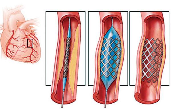
Does the use of stents reduce the risk of strokes?

Read in and view data

stent30 = pd.read_csv("data/stent30.csv")
stent30.head()

	group	outcome
0	treatment	stroke
1	treatment	stroke
2	treatment	stroke
3	treatment	stroke
4	treatment	stroke

Treatment group (N = 224): received stent and medical management (medications, management of risk factors, lifestyle modification)
Control group(N = 227): same medical management as the treatment group, but no stent
Status 30 days after enrollment

What are the hypotheses?

Stents alone prevent strokes
Medical management alone prevents strokes
Both stents and medical management prevent strokes

Why multiple hypotheses?

# Create a frequency table for the 'group' and 'outcome' columns
frequency_table = pd.crosstab(index = stent30['group'], columns = stent30['outcome'])

frequency_table

outcome	no event	stroke
group
control	214	13
treatment	191	33

# Convert frequency table to a proportional table
proportional_table = frequency_table / frequency_table.sum().sum()

proportional_table.round(2)

outcome	no event	stroke
group
control	0.47	0.03
treatment	0.42	0.07

So… does the control affect the occurrence of strokes after 30 days?

Chi-squared test

We need to test the relationship statistically:

# Performing the Chi-Squared Test
chi2, p, dof, expected = chi2_contingency(frequency_table)

print(f"Chi-squared statistic: {chi2.round(2)}")
print(f"P-value: {p.round(3)}")
print(f"Degrees of freedom: {dof}")
print(f"Expected frequencies:\n{expected.round(2)}")

Chi-squared statistic: 9.02
P-value: 0.003
Degrees of freedom: 1
Expected frequencies:
[[203.85  23.15]
 [201.15  22.85]]

Conclusions

There was a >2.5x increase in strokes from the treatment!
There is a statistical difference between no event and strokes when comparing control and treatment groups

BUT! We cannot generalize the results to all patience and all stents.

Data basics

Observations, variables, data matrices

loan50 = pd.read_csv("data/loan50.csv")
loan50.head()

	state	emp_length	term	homeownership	annual_income	verified_income	debt_to_income	total_credit_limit	total_credit_utilized	num_cc_carrying_balance	loan_purpose	loan_amount	grade	interest_rate	public_record_bankrupt	loan_status	has_second_income	total_income
0	NJ	3.0	60	rent	59000.0	Not Verified	0.557525	95131	32894	8	debt_consolidation	22000	B	10.90	0	Current	False	59000.0
1	CA	10.0	36	rent	60000.0	Not Verified	1.305683	51929	78341	2	credit_card	6000	B	9.92	1	Current	False	60000.0
2	SC	NaN	36	mortgage	75000.0	Verified	1.056280	301373	79221	14	debt_consolidation	25000	E	26.30	0	Current	False	75000.0
3	CA	0.0	36	rent	75000.0	Not Verified	0.574347	59890	43076	10	credit_card	6000	B	9.92	0	Current	False	75000.0
4	OH	4.0	60	mortgage	254000.0	Not Verified	0.238150	422619	60490	2	home_improvement	25000	B	9.43	0	Current	False	254000.0

Each row is a case
Each column is a variable
The output is part of a data frame

Metadata

Variable	Description
`loan_amount`	Amount of the loan received, in US dollars.
`interest_rate`	Interest rate on the loan, in an annual percentage.
`term`	The length of the loan, which is always set as a whole number of months.
`grade`	Loan grade, which takes a values A through G and represents the quality of the loan and its likelihood of being repaid.
`state`	US state where the borrower resides.
`total_income`	Borrower’s total income, including any second income, in US dollars.
`homeownership`	Indicates whether the person owns, owns but has a mortgage, or rents.

Types of variables

Types of variables

county = pd.read_csv("data/county.csv")

county.dtypes

name                  object
state                 object
pop2000              float64
pop2010                int64
pop2017              float64
pop_change           float64
poverty              float64
homeownership        float64
multi_unit           float64
unemployment_rate    float64
metro                 object
median_edu            object
per_capita_income    float64
median_hh_income     float64
smoking_ban           object
dtype: object

Relationships between variables

Plot
Code

homeownership (y) and multi_unit (x) have a hypothesized association

Associations

Associations can be negative…

…or positive

Two variables can also not be associated (independent)

Median household income is the explanatory variable
Population change is the response variable
explanatory variable → might affect → response variable

Conclusions

Data should be initially assessed to determine the types of variables
Variables and descriptions are metadata (essential)
Hypothesized associations between the predictor variable and the response variable can be positive, negative, or independent

Study design

Understanding data provenance, including who or what the data represent, is crucial for making comprehensive conclusions.
Sampling is a key aspect of data provenance; knowing how observational units were selected helps generalize findings to the larger population.
Understanding the structure of the study helps distinguish between causal relationships and mere associations.
Before analyzing data, it’s important to ask, “How were these observations collected?” to gain insights about the data’s source and quality.

Sampling principles

Populations and samples

Consider the following:

What is the average mercury content in swordfish in the Atlantic Ocean?
Over the last five years, what is the average time to complete a degree for Duke undergrads?
Does a new drug reduce the number of deaths in patients with severe heart disease?

What does each question have?

Each refers to a target population
Likely not feasible to collect a census of the population
We then collect a sample

Parameters and statistics

Numerical summaries are calculated in each sample or for the entire population
Sample level is a statistic
Population level is a parameter

Anecdotal evidence

Consider the following:

A man on the news got mercury poisoning from eating swordfish, so the average mercury concentration in swordfish must be dangerously high.
I met two students who took more than 7 years to graduate from UArizona, so it must take longer to graduate at UArizona than at many other colleges.
My friend’s dad had a heart attack and died after they gave him a new heart disease drug, so the drug must not work.