Regressions I

Lecture 7

Dr. Greg Chism

University of Arizona
INFO 523 - Spring 2024

Warm up

Announcements

• RQ 3 is due today, 11:59pm

• HW 3 is due today, 11:59pm

• Final project peer-review is Wed Apr 03

Setup

# Import all required libraries
# Data handling and manipulation
import pandas as pd
import numpy as np

# Implementing and selecting models
import statsmodels.api as sm
from sklearn.model_selection import train_test_split, cross_val_score, KFold
from itertools import combinations
from mlxtend.feature_selection import SequentialFeatureSelector as SFS
from sklearn.linear_model import LinearRegression

# For advanced visualizations
import matplotlib.pyplot as plt
import seaborn as sns

# Show computation time
import time

# Increase font size of all Seaborn plot elements
sns.set(font_scale = 1.25)

# Set Seaborn theme
sns.set_theme(style = "white")

Regressions

Linear regression

• Visual
• Definition
• Key points

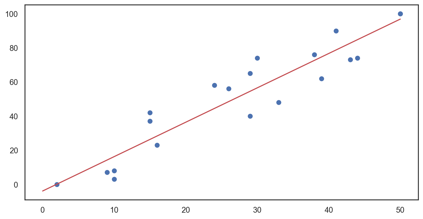
Objective: Minimize the sum of squared differences between observed and predicted.

Model structure:

\(Y_i = \beta_0 + \beta_1 X_i + \epsilon_i\)

• \(Y_i\): Dependent/response variable

• \(X_i\): Independent/predictor variable

• \(\beta_0\): y-intercept

• \(\beta_1\): Slope

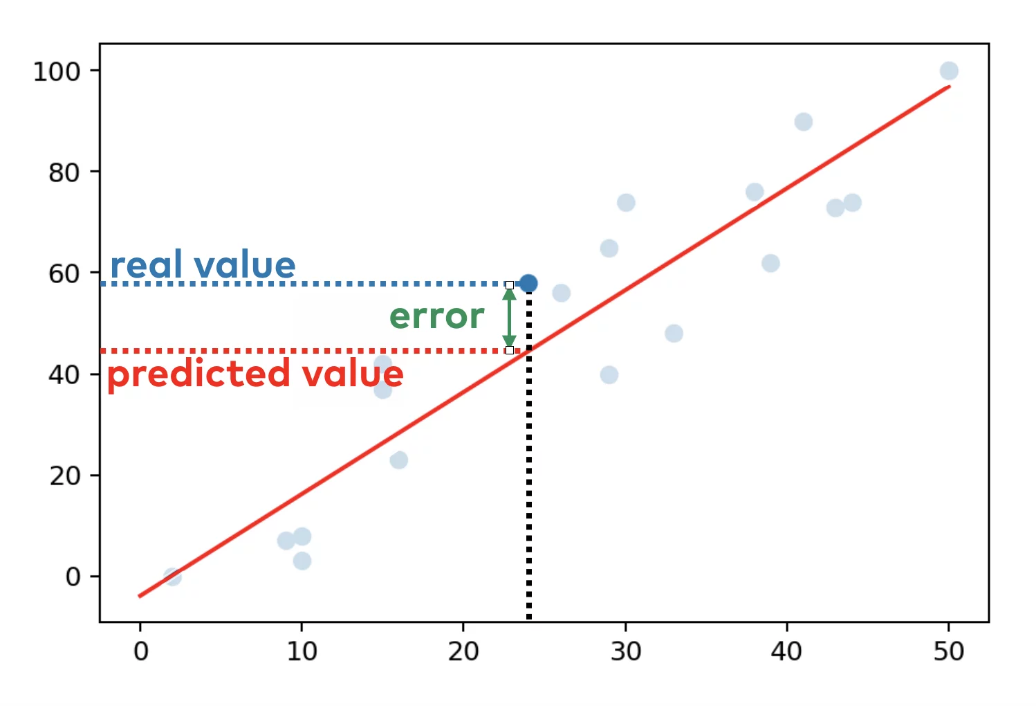
• \(\epsilon_i\): Random error term, deviation of the real value from predicted

1. Assumptions: Linearity, independent residuals, constant variance (homoscedasticity), and normally distributed residuals.

2. Goodness of Fit: Assessed by \(R^2\), the proportion of variance in \(Y\) explained by \(X\).

3. Statistical Significance: Tested by t-tests on the coefficients.

4. Confidence Intervals: Provide a range for the estimated coefficients.

5. Predictions: Use the model to predict \(Y\) for new \(X\) values.

6. Diagnostics: Check residuals for model assumption violations.

7. Sensitivity: Influenced by outliers which can skew the model.

8. Applications: Used across various fields for predictive modeling and data analysis.

Assumptions

Linearity

(Linear relationship between Y ~ X)

Homoscedasticity

(Equal variance among variables)

Multivartiate Normality

(Normally distributed residuals)

Independence

(Observations are independent)

Lack of Multicollinearity

(Predictors are not correlated)

Outlier check

(Technically not an assumption)

Ordinary Least Squares (OLS)

\(\displaystyle y_{i}=\beta_{1} x{i_1}+\beta_{2} x{i_2}+\cdots +\beta_{p} x{i_p}+\varepsilon _{i}\)

1. \(y_i\): Dependent variable for the \(i\)-th observation.
2. \(\beta_1, \beta_2, …, \beta_p\): Coefficients representing the impact of each independent variable.
3. \(x_{i1}, ​x_{i1},…, x_{ip}\): Independent variables for the \(i\)-th observation.
4. \(\epsilon_i\)​: Error term for the \(i\)-th observation, indicating unexplained variance.

Assessing accuracy of coefficients

Two major methods:

1. Standard errors (SE):

• Indicate the precision of coefficient estimates; smaller values suggest more precise estimates.

• Formula: \(\sigma_{\bar{x}} \approx \frac{\sigma_x}{\sqrt{n}}\)

2. Confidence Intervals:

• Ranges constructed from standard errors that indicate where the true coefficient is likely to fall, typically at a 95% confidence level.

• Derived from same method as p-values

Assessing accuracy of model

• Overview
• MSE
• R-squared
• Adjusted R-squared
• Residual plots

Four major methods:

1. Mean square error (MSE): MSE of a predictor is calculated as the average of the squares of the errors, where the error is the difference between the actual value and the predicted value.
2. R-squared (\(R^2\)): Proportion of variance in the dependent variable explained by the model; closer to 1 indicates a better fit.
3. Adjusted R-squared (\(R^2_{adj}\)): Modified R² that accounts for the number of predictors; useful for comparing models with different numbers of independent variables.
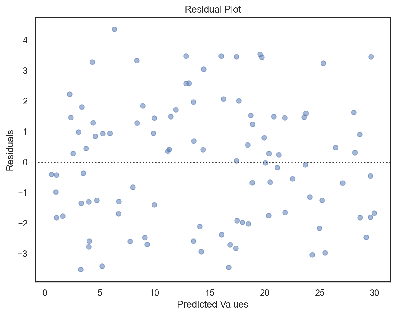
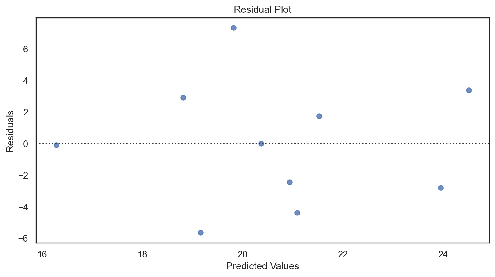
4. Residual plots: Visual check for randomness in residuals; patterns may indicate model issues like non-linearity or heteroscedasticity.

In statistics, the mean squared error (MSE) or mean squared deviation (MSD) of an estimator measures the average of the squares of the errors—that is, the average squared difference between the estimated values and the actual value. The MSE either assesses the quality of a predictoror of an estimator.

Predictor

\(MSE = \frac{1}{n} \sum_{i=1}^{n} (y_i - \hat{y}_i)^2\)

• \(y_i\): the actual values

• \(\hat{y}_i\): the predicted values

• \(n\): sample size

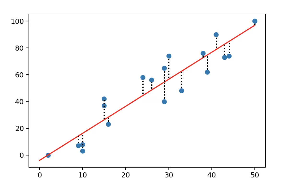
Define the residuals as \(e_i = y_i − f_i\)(forming a vector \(e\)).

If \(\bar{y}\) is the observed mean:

\(\bar{y}=\frac{1}{n} \sum_{i=1}^{n}y_i\)

then the variability of the data set can be measured with two sums of squares (SS) formulas:

Residual SS:

\(RSS = \sum_{i=1}^{n} (y_i - \hat{y}_i)^2\)

Total SS:

\(TSS = \sum_{i=1}^{n} (y_i - \bar{y})^2\)

R-squared:

\(R^2 = 1 - \frac{RSS}{TSS}\)

Formula \(R^2 = 1 - \frac{RSS / df_{res}}{TSS / df_{tot}}\)

Key points:

• Penalizes Complexity: Adjusts for the number of terms in the model, penalizing the addition of irrelevant predictors.

• Comparability: More reliable than R-squared for comparing models with different numbers of independent variables.

• Value Range: Can be negative if the model is worse than using just the mean of the dependent variable, whereas R-squared is always between 0 and 1.

• \(df_{res}\): degrees of freedom of the estimate of the population variance around the model
• \(df_{tot}\): degrees of freedom of the estimate of the population variance around the mean

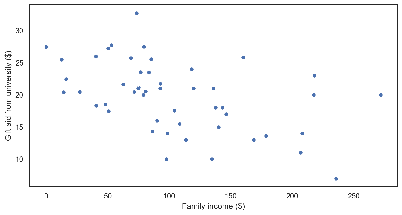
Our data

• Read
• Info
• Describe
• Plot

elmhurst = pd.read_csv("data/elmhurst.csv")

elmhurst.info()

<class 'pandas.core.frame.DataFrame'>
RangeIndex: 50 entries, 0 to 49
Data columns (total 3 columns):
 #   Column         Non-Null Count  Dtype  
---  ------         --------------  -----  
 0   family_income  50 non-null     float64
 1   gift_aid       50 non-null     float64
 2   price_paid     50 non-null     float64
dtypes: float64(3)
memory usage: 1.3 KB

elmhurst.describe()

	family_income	gift_aid	price_paid
count	50.000000	50.000000	50.000000
mean	101.778520	19.935560	19.544440
std	63.206451	5.460581	5.979759
min	0.000000	7.000000	8.530000
25%	64.079000	16.250000	15.000000
50%	88.061500	20.470000	19.500000
75%	137.174000	23.515000	23.630000
max	271.974000	32.720000	35.000000

sns.scatterplot(data = elmhurst, x = "family_income", y = "gift_aid")
plt.xlabel("Family income ($)")
plt.ylabel("Gift aid from university ($)")
plt.show()

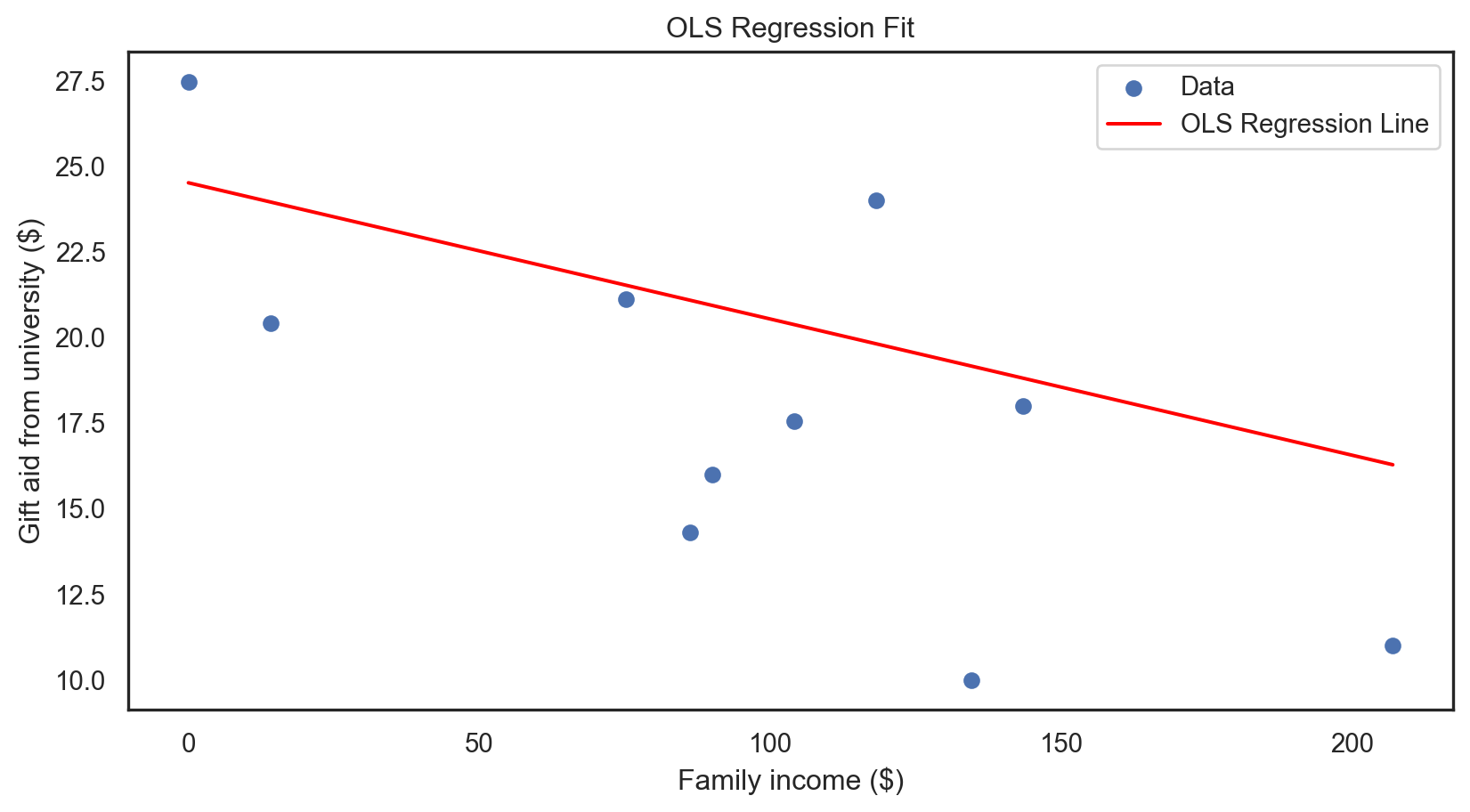
OLS regression: applied

• Model summary
• Residual plot
• Regression fit plot

Code

X = elmhurst['family_income']  # Independent variable
y = elmhurst['gift_aid']  # Dependent variable

X_train, X_test, y_train, y_test = train_test_split(X, y, test_size = 0.2, random_state = 42)
X_train_with_const = sm.add_constant(X_train)

model = sm.OLS(y_train, X_train_with_const).fit()

model_summary2 = model.summary2()
print(model_summary2)

                 Results: Ordinary least squares
=================================================================
Model:              OLS              Adj. R-squared:     0.205   
Dependent Variable: gift_aid         AIC:                241.3545
Date:               2024-04-25 15:09 BIC:                244.7323
No. Observations:   40               Log-Likelihood:     -118.68 
Df Model:           1                F-statistic:        11.05   
Df Residuals:       38               Prob (F-statistic): 0.00197 
R-squared:          0.225            Scale:              23.273  
-----------------------------------------------------------------
                   Coef.  Std.Err.    t    P>|t|   [0.025  0.975]
-----------------------------------------------------------------
const             24.5170   1.4489 16.9216 0.0000 21.5839 27.4500
family_income     -0.0398   0.0120 -3.3238 0.0020 -0.0640 -0.0156
-----------------------------------------------------------------
Omnibus:              0.057        Durbin-Watson:           2.277
Prob(Omnibus):        0.972        Jarque-Bera (JB):        0.249
Skew:                 0.047        Prob(JB):                0.883
Kurtosis:             2.625        Condition No.:           230  
=================================================================
Notes:
[1] Standard Errors assume that the covariance matrix of the
errors is correctly specified.

Code

X_test_with_const = sm.add_constant(X_test)
predictions = model.predict(X_test_with_const)
residuals = y_test - predictions

sns.residplot(x = predictions, y = residuals)
plt.xlabel('Predicted Values')
plt.ylabel('Residuals')
plt.title('Residual Plot')
plt.show()

Code

plt.scatter(X_test, y_test, label = 'Data')

line_x = np.linspace(X_test.min(), X_test.max(), 100)
line_y = model.predict(sm.add_constant(line_x))
plt.plot(line_x, line_y, color = 'red', label = 'OLS Regression Line')

plt.xlabel("Family income ($)")
plt.ylabel("Gift aid from university ($)")
plt.title('OLS Regression Fit')
plt.legend()
plt.show()

Multiple regression

Multiple regression

• Visual
• Key points

1. Multiple Predictors: more than one predictor variable to predict a response variable.

2. Model Form: \(Y = \beta_0 + \beta_1 X_1 + \beta_2 X_2 + \cdots + \beta_n X_n + \epsilon\) , where \(Y\) is the response variable, \(X_1, X_2,...,X_n\) are predictor variables, \(\beta\)s are coefficients, and \(\epsilon\) is the error term.

3. Coefficient Interpretation: Each coefficient represents the change in the response variable for one unit change in the predictor, holding other predictors constant.

4. Assumptions: Includes linearity, no perfect multicollinearity, homoscedasticity, independence of errors, and normality of residuals.

5. Adjusted R-squared: Used to determine the model’s explanatory power, adjusting for the number of predictors.

6. Multicollinearity Concerns: High correlation between predictor variables can distort the model and make coefficient estimates unreliable.

7. Interaction Effects: Can be included to see if the effect of one predictor on the response variable depends on another predictor.

Our data

• Question
• Read + examine
• Relevant variables
• Info
• Describe
• Plot

How do factors like debt-to-income ratio, bankruptcy history, and loan term affect the interest rate of a loan?

loans = pd.read_csv("data/loans.csv")
loans.head()

	emp_title	emp_length	state	homeownership	annual_income	verified_income	debt_to_income	annual_income_joint	verification_income_joint	debt_to_income_joint	...	sub_grade	issue_month	loan_status	initial_listing_status	disbursement_method	balance	paid_total	paid_principal	paid_interest	paid_late_fees
0	global config engineer	3.0	NJ	MORTGAGE	90000.0	Verified	18.01	NaN	NaN	NaN	...	C3	Mar-2018	Current	whole	Cash	27015.86	1999.33	984.14	1015.19	0.0
1	warehouse office clerk	10.0	HI	RENT	40000.0	Not Verified	5.04	NaN	NaN	NaN	...	C1	Feb-2018	Current	whole	Cash	4651.37	499.12	348.63	150.49	0.0
2	assembly	3.0	WI	RENT	40000.0	Source Verified	21.15	NaN	NaN	NaN	...	D1	Feb-2018	Current	fractional	Cash	1824.63	281.80	175.37	106.43	0.0
3	customer service	1.0	PA	RENT	30000.0	Not Verified	10.16	NaN	NaN	NaN	...	A3	Jan-2018	Current	whole	Cash	18853.26	3312.89	2746.74	566.15	0.0
4	security supervisor	10.0	CA	RENT	35000.0	Verified	57.96	57000.0	Verified	37.66	...	C3	Mar-2018	Current	whole	Cash	21430.15	2324.65	1569.85	754.80	0.0

5 rows × 55 columns

Variable	Description
interest_rate	Interest rate on the loan, in an annual percentage.
verified_income	Borrower’s income verification: Verified, Source Verified, and Not Verified.
debt_to_income	Debt-to-income ratio, which is the percentage of total debt of the borrower divided by their total income.
credit_util	The fraction of available credit utilized.
bankruptcy	An indicator variable for whether the borrower has a past bankruptcy in their record. This variable takes a value of 1 if the answer is yes and 0 if the answer is no.
term	The length of the loan, in months.
issue_month	The month and year the loan was issued.
credit_checks	Number of credit checks in the last 12 months.

loans.info()

<class 'pandas.core.frame.DataFrame'>
RangeIndex: 10000 entries, 0 to 9999
Data columns (total 55 columns):
 #   Column                            Non-Null Count  Dtype  
---  ------                            --------------  -----  
 0   emp_title                         9167 non-null   object 
 1   emp_length                        9183 non-null   float64
 2   state                             10000 non-null  object 
 3   homeownership                     10000 non-null  object 
 4   annual_income                     10000 non-null  float64
 5   verified_income                   10000 non-null  object 
 6   debt_to_income                    9976 non-null   float64
 7   annual_income_joint               1495 non-null   float64
 8   verification_income_joint         1455 non-null   object 
 9   debt_to_income_joint              1495 non-null   float64
 10  delinq_2y                         10000 non-null  int64  
 11  months_since_last_delinq          4342 non-null   float64
 12  earliest_credit_line              10000 non-null  int64  
 13  inquiries_last_12m                10000 non-null  int64  
 14  total_credit_lines                10000 non-null  int64  
 15  open_credit_lines                 10000 non-null  int64  
 16  total_credit_limit                10000 non-null  int64  
 17  total_credit_utilized             10000 non-null  int64  
 18  num_collections_last_12m          10000 non-null  int64  
 19  num_historical_failed_to_pay      10000 non-null  int64  
 20  months_since_90d_late             2285 non-null   float64
 21  current_accounts_delinq           10000 non-null  int64  
 22  total_collection_amount_ever      10000 non-null  int64  
 23  current_installment_accounts      10000 non-null  int64  
 24  accounts_opened_24m               10000 non-null  int64  
 25  months_since_last_credit_inquiry  8729 non-null   float64
 26  num_satisfactory_accounts         10000 non-null  int64  
 27  num_accounts_120d_past_due        9682 non-null   float64
 28  num_accounts_30d_past_due         10000 non-null  int64  
 29  num_active_debit_accounts         10000 non-null  int64  
 30  total_debit_limit                 10000 non-null  int64  
 31  num_total_cc_accounts             10000 non-null  int64  
 32  num_open_cc_accounts              10000 non-null  int64  
 33  num_cc_carrying_balance           10000 non-null  int64  
 34  num_mort_accounts                 10000 non-null  int64  
 35  account_never_delinq_percent      10000 non-null  float64
 36  tax_liens                         10000 non-null  int64  
 37  public_record_bankrupt            10000 non-null  int64  
 38  loan_purpose                      10000 non-null  object 
 39  application_type                  10000 non-null  object 
 40  loan_amount                       10000 non-null  int64  
 41  term                              10000 non-null  int64  
 42  interest_rate                     10000 non-null  float64
 43  installment                       10000 non-null  float64
 44  grade                             10000 non-null  object 
 45  sub_grade                         10000 non-null  object 
 46  issue_month                       10000 non-null  object 
 47  loan_status                       10000 non-null  object 
 48  initial_listing_status            10000 non-null  object 
 49  disbursement_method               10000 non-null  object 
 50  balance                           10000 non-null  float64
 51  paid_total                        10000 non-null  float64
 52  paid_principal                    10000 non-null  float64
 53  paid_interest                     10000 non-null  float64
 54  paid_late_fees                    10000 non-null  float64
dtypes: float64(17), int64(25), object(13)
memory usage: 4.2+ MB

loans.describe()

	emp_length	annual_income	debt_to_income	annual_income_joint	debt_to_income_joint	delinq_2y	months_since_last_delinq	earliest_credit_line	inquiries_last_12m	total_credit_lines	...	public_record_bankrupt	loan_amount	term	interest_rate	installment	balance	paid_total	paid_principal	paid_interest	paid_late_fees
count	9183.000000	1.000000e+04	9976.000000	1.495000e+03	1495.000000	10000.00000	4342.000000	10000.00000	10000.00000	10000.000000	...	10000.000000	10000.000000	10000.000000	10000.000000	10000.000000	10000.000000	10000.000000	10000.000000	10000.000000	10000.000000
mean	5.930306	7.922215e+04	19.308192	1.279146e+05	19.979304	0.21600	36.760709	2001.29000	1.95820	22.679600	...	0.123800	16361.922500	43.272000	12.427524	476.205323	14458.916610	2494.234773	1894.448466	599.666781	0.119516
std	3.703734	6.473429e+04	15.004851	7.016838e+04	8.054781	0.68366	21.634939	7.79551	2.38013	11.885439	...	0.337172	10301.956759	11.029877	5.001105	294.851627	9964.561865	3958.230365	3884.407175	517.328062	1.813468
min	0.000000	0.000000e+00	0.000000	1.920000e+04	0.320000	0.00000	1.000000	1963.00000	0.00000	2.000000	...	0.000000	1000.000000	36.000000	5.310000	30.750000	0.000000	0.000000	0.000000	0.000000	0.000000
25%	2.000000	4.500000e+04	11.057500	8.683350e+04	14.160000	0.00000	19.000000	1997.00000	0.00000	14.000000	...	0.000000	8000.000000	36.000000	9.430000	256.040000	6679.065000	928.700000	587.100000	221.757500	0.000000
50%	6.000000	6.500000e+04	17.570000	1.130000e+05	19.720000	0.00000	34.000000	2003.00000	1.00000	21.000000	...	0.000000	14500.000000	36.000000	11.980000	398.420000	12379.495000	1563.300000	984.990000	446.140000	0.000000
75%	10.000000	9.500000e+04	25.002500	1.515455e+05	25.500000	0.00000	53.000000	2006.00000	3.00000	29.000000	...	0.000000	24000.000000	60.000000	15.050000	644.690000	20690.182500	2616.005000	1694.555000	825.420000	0.000000
max	10.000000	2.300000e+06	469.090000	1.100000e+06	39.980000	13.00000	118.000000	2015.00000	29.00000	87.000000	...	3.000000	40000.000000	60.000000	30.940000	1566.590000	40000.000000	41630.443684	40000.000000	4216.440000	52.980000

8 rows × 42 columns

Code

sns.scatterplot(data = loans, x = "debt_to_income", y = "interest_rate", hue = "loan_purpose")
plt.xlabel("Annual income ($)")
plt.ylabel("Loan interest rate (%)")
plt.legend(title = "Loan purpose")
plt.show()

Our data: preprocessed

loans['credit_util'] = loans['total_credit_utilized'] / loans['total_credit_limit']
loans['bankruptcy'] = (loans['public_record_bankrupt'] != 0).astype(int)
loans['verified_income'] = loans['verified_income'].astype('category').cat.remove_unused_categories()
loans = loans.rename(columns = {'inquiries_last_12m': 'credit_checks'})

loans = loans[['interest_rate', 'verified_income', 'debt_to_income', 'credit_util', 'bankruptcy', 'term', 'credit_checks', 'issue_month']]

Multiple regression: applied

• Model summary
• Coefficients
• Residual plot
• Regression fit

Code

X = loans[['verified_income', 'debt_to_income', 'credit_util', 'bankruptcy', 'term', 'credit_checks', 'issue_month']]  
y = loans['interest_rate']  
X = pd.get_dummies(X, columns = ['verified_income', 'issue_month'], drop_first = True)
X.fillna(0, inplace=True)

X_train, X_test, y_train, y_test = train_test_split(X, y, test_size = 0.2, random_state = 42)

X_train_with_const = sm.add_constant(X_train)
X_test_with_const = sm.add_constant(X_test)

X_train_with_const = X_train_with_const.astype(int)
X_test_with_const = X_test_with_const.astype(int)

model = sm.OLS(y_train, X_train_with_const).fit()

model_summary2 = model.summary2()
print(model_summary2)

                       Results: Ordinary least squares
==============================================================================
Model:                   OLS                 Adj. R-squared:        0.191     
Dependent Variable:      interest_rate       AIC:                   46653.7930
Date:                    2024-04-25 15:09    BIC:                   46723.6650
No. Observations:        8000                Log-Likelihood:        -23317.   
Df Model:                9                   F-statistic:           210.4     
Df Residuals:            7990                Prob (F-statistic):    0.00      
R-squared:               0.192               Scale:                 19.937    
------------------------------------------------------------------------------
                                 Coef.  Std.Err.    t    P>|t|   [0.025 0.975]
------------------------------------------------------------------------------
const                            4.0713   0.2319 17.5583 0.0000  3.6167 4.5258
debt_to_income                   0.0330   0.0033  9.8715 0.0000  0.0265 0.0396
credit_util                      3.0409   0.4077  7.4585 0.0000  2.2417 3.8401
bankruptcy                       0.5811   0.1543  3.7659 0.0002  0.2786 0.8836
term                             0.1445   0.0046 31.5795 0.0000  0.1356 0.1535
credit_checks                    0.2122   0.0211 10.0534 0.0000  0.1708 0.2535
verified_income_Source Verified  1.0041   0.1150  8.7304 0.0000  0.7787 1.2296
verified_income_Verified         2.4460   0.1355 18.0457 0.0000  2.1803 2.7117
issue_month_Jan-2018            -0.0778   0.1254 -0.6204 0.5350 -0.3236 0.1680
issue_month_Mar-2018            -0.0178   0.1233 -0.1445 0.8851 -0.2596 0.2239
------------------------------------------------------------------------------
Omnibus:                  762.745          Durbin-Watson:             1.958   
Prob(Omnibus):            0.000            Jarque-Bera (JB):          1001.147
Skew:                     0.820            Prob(JB):                  0.000   
Kurtosis:                 3.562            Condition No.:             398     
==============================================================================
Notes:
[1] Standard Errors assume that the covariance matrix of the errors is
correctly specified.

\[\begin{aligned} \widehat{\texttt{interest\_rate}} &= b_0 \\ &+ b_1 \times \texttt{verified\_income}_{\texttt{Source Verified}} \\ &+ b_2 \times \texttt{verified\_income}_{\texttt{Verified}} \\ &+ b_3 \times \texttt{debt\_to\_income} \\ &+ b_4 \times \texttt{credit\_util} \\ &+ b_5 \times \texttt{bankruptcy} \\ &+ b_6 \times \texttt{term} \\ &+ b_9 \times \texttt{credit\_checks} \\ &+ b_7 \times \texttt{issue\_month}_{\texttt{Jan-2018}} \\ &+ b_8 \times \texttt{issue\_month}_{\texttt{Mar-2018}} \end{aligned}\]

Code

X_test_with_const = sm.add_constant(X_test)
predictions = model.predict(X_test_with_const)
predictions = pd.to_numeric(predictions, errors='coerce')
residuals = y_test - predictions
residuals = pd.to_numeric(residuals, errors='coerce').fillna(0)

# Plotting the residuals
sns.residplot(x = predictions, y = residuals)
plt.xlabel('Predicted Values')
plt.ylabel('Residuals')
plt.title('Residual Plot')
plt.show()

Code

plt.scatter(predictions, y_test, label = 'Data')
plt.plot(y_test, y_test, color = 'red', label = 'Ideal Fit')  

plt.xlabel('Predicted Interest Rate')
plt.ylabel('Actual Interest Rate')
plt.title('Multiple Regression Fit')
plt.legend()
plt.show()

Model optimization

• Overview
• AIC
• BIC
• k-Fold CV

Three major methods:

1. AIC (Akaike Information Criterion): a measure of the relative quality of a statistical model for a given set of data. Lower and fewer parameters = better.
   • \(AIC=2k−2\ln(L)\), where \(k\) is the number of parameters, and \(L\) is the likelihood of the model.
2. BIC (Bayesian Information Criterion): a criterion for model selection based on the likelihood of the model. Lower and fewer parameters = better.
   • \(BIC = k \ln(n) - 2 \ln(L)\), where \(k\) is the number of parameters, \(n\) is the sample size, and \(L\) is the likelihood of the model
3. Cross-Validation: a statistical method used for assessing how the results of a predictive model will generalize to an independent data set.
   • Most common method is k-Fold Cross Validation

Pros:

1. Balanced Approach: AIC balances model fit with complexity, reducing overfitting.

2. Comparative Utility: Suitable for comparing models on the same dataset.

3. Widespread Acceptance: Commonly used and recognized in statistical analysis.

4. Versatile: Applicable across various types of statistical models.

Cons:

1. Relative Measurement: Only provides a comparative metric and doesn’t indicate absolute model quality.

2. Risk of Underfitting: Penalizing complex models may lead to underfitting.

3. Sample Size Sensitivity: Its effectiveness can vary with the size of the dataset.

4. Assumption of Large Sample: Infinite sample size assumption is impractical.

5. No Probabilistic Interpretation: Lacks a direct probabilistic meaning, unlike some other statistical measures.

Pros:

1. Penalizes Complexity: Penalizes complexity, preventing overfitting.

2. Good for Large Data: The penalty term is more significant in larger datasets.

3. Model Comparison: Useful for comparing different models on the same dataset.

4. Widely Recognized: Commonly used in statistical model selection.

Cons:

1. Relative, Not Absolute: Only provides a comparative metric and doesn’t indicate absolute model quality.

2. Can Favor Simpler Models: Penalizing complex models may lead to underfitting.

3. Sample Size Dependent: The effectiveness of BIC is influenced by sample size.

4. Assumes Correct Model is in Set: Assumes that the true model is given.

5. Lacks Probabilistic Meaning: Lacks a direct probabilistic meaning, unlike some other statistical measures.

Pros:

1. Robustness: Provides a more accurate measure of out-of-sample accuracy.

2. Prevents Overfitting: Helps in detecting overfitting by evaluating model performance on unseen data.

3. Versatile: Can be used with any predictive modeling technique.

4. Tuning Hyperparameters: Useful for selecting the best model hyperparameters.

Cons:

1. Computationally Intensive: Can be slow with large datasets and complex models.

2. Data Requirements: Requires a sufficient amount of data to partition into meaningful subsets.

3. Variance: Results can be sensitive to the way in which data is divided.

4. No Single Best Model: only provides an estimation of how well a model type will perform.

Model selection

Model selection

The task of selecting a model from among various candidates on the basis of performance criterion to choose the best one.

Two major methods:

1. Best subset selection: Evaluate all combinations, choose by a criterion - e.g., lowest \(RSS\) or highest \(R^{2}_{adj}\)
2. Stepwise selection: Forward Selection or Backward Selection

Best subset selection

• Overview
• Formula
• Pros + cons

Definition

Best Subset Selection is a statistical method used in regression analysis to select a subset of predictors that provides the best fit for the response variable.

It involves:

1. Considering All Possible Predictor Subsets: For \(p\) predictors, all possible combinations (totaling \(2_p\)) of these predictors are considered.

2. Fitting a Model for Each Subset: A regression model is fitted for each subset of predictors.

3. Selecting the Best Model: The best model is selected based on a criterion that balances fit and complexity, such as the lowest Residual Sum of Squares (\(RSS\)) or the highest \(R^{2}_{adj}\) (or \(AIC\), \(BIC\)).

For each subset, the model is given by:

\(Y = \beta_0 + \sum_{i \in S} \beta_i X_i + \epsilon\)

• \(Y\): Response variable.

• \(\beta_0\): Intercept.

• \(\beta_i\): Coefficients for predictors.

• \(X_i\): Predictor variables.

• \(\epsilon\): Error term.

• \(S\): Set of indices of selected predictors.

The quality of each model is assessed using a criterion like:

\(RSS = \sum_{i=1}^{n} (y_i - \hat{y}_i)^2\)

…or \(R^{2}_{adj}\),\(AIC\),\(BIC\)

Pros:

1. Comprehensive Approach: Evaluates all possible combinations of predictors, ensuring a thorough search.

2. Flexibility: Can be used with various selection criteria and types of regression models.

3. Intuitive: Provides a clear framework for model selection.

Cons:

1. Computational Intensity: The number of models to evaluate grows exponentially with the number of predictors, making it computationally demanding.

2. Overfitting Risk: May lead to overfit models, especially when the number of observations is not significantly larger than the number of predictors.

3. Model Selection Complexity: Requires careful choice and interpretation of model selection criteria to balance between model fit and complexity.

Stepwise selection (both types)

• Overview
• Formula
• Pros + cons

Definition

Stepwise selection is a method used in regression analysis to select predictor variables. There are two main types:

Forward Selection:

1. Starts with no predictor variables in the model.

2. Iteratively adds the variable that provides the most significant model improvement.

3. Continues until no significant improvement is made by adding more variables.

Backward Selection:

1. Begins with all candidate predictor variables.

2. Iteratively removes the least significant variable (that least worsens the model).

3. Continues until removing more variables significantly worsens the model.

The criteria for adding or removing a variable are usually based on statistical tests like the F-test or p-values:

Forward selection (adding a variable)

\(F = \frac{(\text{RSS}_0 - \text{RSS}_1) / p_1}{\text{RSS}_1 / (n - p_0 - 1)}\)

• \(RSS_0\) is the Residual Sum of Squares of the current model.
• \(RSS_1\) is the Residual Sum of Squares with the additional variable.
• \(p_1\) is the number of predictors in the new model.
• \(n\) is the number of observations.
• \(p_0\) is the number of predictors in the current model.

Backward selection (removing a variable)

Similar criteria but in reverse, considering the increase in \(RSS\) or the p-values of the coefficients.

Pros:

1. Simplicity: More straightforward and computationally less intensive than Best Subset Selection.

2. Flexibility: Can be adapted to various criteria for entering and removing variables.

3. Practical: Useful with multicollinearity and large sets of potential predictors.

Cons:

1. Arbitrary Choices: Depends on the order of variables and the specific entry and removal criteria.

2. Local Optima: Might not find the best possible model as it doesn’t evaluate all possible combinations.

3. Overfitting Risk: Especially in datasets with many variables relative to the number of observations.

4. Statistical Issues: Stepwise methods can inflate the significance of variables and do not account for the search process in assessing the fit.

Best Subset Selection: applied

• Original
• Implementing BSS
• AIC
• BIC
• \(R^{2}_{adj}\)

Code

X = loans[['verified_income', 'debt_to_income', 'credit_util', 'bankruptcy', 'term', 'credit_checks', 'issue_month']]  
y = loans['interest_rate']  
X = pd.get_dummies(X, columns = ['verified_income', 'issue_month'], drop_first = True)
X.fillna(0, inplace=True)

X_train, X_test, y_train, y_test = train_test_split(X, y, test_size = 0.2, random_state = 42)

X_train_with_const = sm.add_constant(X_train)
X_test_with_const = sm.add_constant(X_test)

X_train_with_const = X_train_with_const.astype(int)
X_test_with_const = X_test_with_const.astype(int)

model = sm.OLS(y_train, X_train_with_const).fit()

model_summary2 = model.summary2()
print(model_summary2)

                       Results: Ordinary least squares
==============================================================================
Model:                   OLS                 Adj. R-squared:        0.191     
Dependent Variable:      interest_rate       AIC:                   46653.7930
Date:                    2024-04-25 15:09    BIC:                   46723.6650
No. Observations:        8000                Log-Likelihood:        -23317.   
Df Model:                9                   F-statistic:           210.4     
Df Residuals:            7990                Prob (F-statistic):    0.00      
R-squared:               0.192               Scale:                 19.937    
------------------------------------------------------------------------------
                                 Coef.  Std.Err.    t    P>|t|   [0.025 0.975]
------------------------------------------------------------------------------
const                            4.0713   0.2319 17.5583 0.0000  3.6167 4.5258
debt_to_income                   0.0330   0.0033  9.8715 0.0000  0.0265 0.0396
credit_util                      3.0409   0.4077  7.4585 0.0000  2.2417 3.8401
bankruptcy                       0.5811   0.1543  3.7659 0.0002  0.2786 0.8836
term                             0.1445   0.0046 31.5795 0.0000  0.1356 0.1535
credit_checks                    0.2122   0.0211 10.0534 0.0000  0.1708 0.2535
verified_income_Source Verified  1.0041   0.1150  8.7304 0.0000  0.7787 1.2296
verified_income_Verified         2.4460   0.1355 18.0457 0.0000  2.1803 2.7117
issue_month_Jan-2018            -0.0778   0.1254 -0.6204 0.5350 -0.3236 0.1680
issue_month_Mar-2018            -0.0178   0.1233 -0.1445 0.8851 -0.2596 0.2239
------------------------------------------------------------------------------
Omnibus:                  762.745          Durbin-Watson:             1.958   
Prob(Omnibus):            0.000            Jarque-Bera (JB):          1001.147
Skew:                     0.820            Prob(JB):                  0.000   
Kurtosis:                 3.562            Condition No.:             398     
==============================================================================
Notes:
[1] Standard Errors assume that the covariance matrix of the errors is
correctly specified.

def best_subset_selection(X, y):
    results = []
    for k in range(1, len(X.columns) + 1):
        for combo in combinations(X.columns, k):
            X_subset = sm.add_constant(X[list(combo)].astype(int))
            model = sm.OLS(y, X_subset).fit()
            results.append({'model': model, 'predictors': combo})
    return results

subset_results = best_subset_selection(X_train, y_train)

best_aic = np.inf
best_model_1 = None

for result in subset_results:
    if result['model'].aic < best_aic:
        best_aic = result['model'].aic
        best_model_1 = result
        
print("Best Model Predictors:", best_model_1['predictors'])
print("Best Model AIC:", best_aic.round(2))

Best Model Predictors: ('debt_to_income', 'credit_util', 'bankruptcy', 'term', 'credit_checks', 'verified_income_Source Verified', 'verified_income_Verified')
Best Model AIC: 46650.23

best_bic = np.inf
best_model_2 = None

for result in subset_results:
    if result['model'].bic < best_bic:
        best_bic = result['model'].bic
        best_model_2 = result
        
print("Best Model Predictors:", best_model_2['predictors'])
print("Best Model BIC:", best_bic.round(2))

Best Model Predictors: ('debt_to_income', 'credit_util', 'bankruptcy', 'term', 'credit_checks', 'verified_income_Source Verified', 'verified_income_Verified')
Best Model BIC: 46706.13

best_r_sq_adj = -np.inf  
best_model_3 = None

for result in subset_results:
    if result['model'].rsquared_adj > best_r_sq_adj:  
        best_r_sq_adj = result['model'].rsquared_adj
        best_model_3 = result
        
print("Best Model Predictors:", best_model_3['predictors'])
print("Best Model Adjusted R-squared:", best_r_sq_adj.round(2))

Best Model Predictors: ('debt_to_income', 'credit_util', 'bankruptcy', 'term', 'credit_checks', 'verified_income_Source Verified', 'verified_income_Verified')
Best Model Adjusted R-squared: 0.19

Step-wise selection: applied

• Original
• Forward selection
• Backward selection

Code

X = loans[['verified_income', 'debt_to_income', 'credit_util', 'bankruptcy', 'term', 'credit_checks', 'issue_month']]  
y = loans['interest_rate']  
X = pd.get_dummies(X, columns = ['verified_income', 'issue_month'], drop_first = True)
X.fillna(0, inplace=True)

X_train, X_test, y_train, y_test = train_test_split(X, y, test_size = 0.2, random_state = 42)

X_train_with_const = sm.add_constant(X_train)
X_test_with_const = sm.add_constant(X_test)

X_train_with_const = X_train_with_const.astype(int)
X_test_with_const = X_test_with_const.astype(int)

model = sm.OLS(y_train, X_train_with_const).fit()

model_summary2 = model.summary2()
print(model_summary2)

                       Results: Ordinary least squares
==============================================================================
Model:                   OLS                 Adj. R-squared:        0.191     
Dependent Variable:      interest_rate       AIC:                   46653.7930
Date:                    2024-04-25 15:09    BIC:                   46723.6650
No. Observations:        8000                Log-Likelihood:        -23317.   
Df Model:                9                   F-statistic:           210.4     
Df Residuals:            7990                Prob (F-statistic):    0.00      
R-squared:               0.192               Scale:                 19.937    
------------------------------------------------------------------------------
                                 Coef.  Std.Err.    t    P>|t|   [0.025 0.975]
------------------------------------------------------------------------------
const                            4.0713   0.2319 17.5583 0.0000  3.6167 4.5258
debt_to_income                   0.0330   0.0033  9.8715 0.0000  0.0265 0.0396
credit_util                      3.0409   0.4077  7.4585 0.0000  2.2417 3.8401
bankruptcy                       0.5811   0.1543  3.7659 0.0002  0.2786 0.8836
term                             0.1445   0.0046 31.5795 0.0000  0.1356 0.1535
credit_checks                    0.2122   0.0211 10.0534 0.0000  0.1708 0.2535
verified_income_Source Verified  1.0041   0.1150  8.7304 0.0000  0.7787 1.2296
verified_income_Verified         2.4460   0.1355 18.0457 0.0000  2.1803 2.7117
issue_month_Jan-2018            -0.0778   0.1254 -0.6204 0.5350 -0.3236 0.1680
issue_month_Mar-2018            -0.0178   0.1233 -0.1445 0.8851 -0.2596 0.2239
------------------------------------------------------------------------------
Omnibus:                  762.745          Durbin-Watson:             1.958   
Prob(Omnibus):            0.000            Jarque-Bera (JB):          1001.147
Skew:                     0.820            Prob(JB):                  0.000   
Kurtosis:                 3.562            Condition No.:             398     
==============================================================================
Notes:
[1] Standard Errors assume that the covariance matrix of the errors is
correctly specified.

Code

lr = LinearRegression()

# Initialize SequentialFeatureSelector (SFS) for forward selection
sfs = SFS(lr, 
          k_features = 'best',  # Select the best number of features based on criterion
          forward = True,  # Forward selection
          floating = False,
          scoring = 'neg_mean_squared_error',  # Using negative MSE as scoring criterion
          cv = 0)  # No cross-validation

# Fit SFS on the training data
sfs.fit(X_train, y_train)

# Get the names of the selected features
selected_features = list(sfs.k_feature_names_)

# Convert the DataFrame to numeric to ensure all features are numeric
X_train = X_train.apply(pd.to_numeric, errors='coerce').fillna(0)
X_test = X_test.apply(pd.to_numeric, errors='coerce').fillna(0)

# Select the features identified by forward selection
X_train_selected = X_train[selected_features]

# Fit the final Linear Regression model using selected features
final_model = lr.fit(X_train_selected, y_train)

# For AIC, BIC, and adjusted R-squared, use statsmodels
X_train_selected_with_const = sm.add_constant(X_train_selected)

# Ensure data type consistency
X_train_selected_with_const = X_train_selected_with_const.astype(float)

# Fit the OLS model
model_sm = sm.OLS(y_train, X_train_selected_with_const).fit()

# Output the results
print("Forward Selection Results")
print("Selected predictors:", selected_features)
print("AIC:", model_sm.aic.round(3))
print("BIC:", model_sm.bic.round(3))
print("Adjusted R-squared:", model_sm.rsquared_adj.round(3))

Forward Selection Results
Selected predictors: ['debt_to_income', 'credit_util', 'bankruptcy', 'term', 'credit_checks', 'verified_income_Source Verified', 'verified_income_Verified', 'issue_month_Jan-2018', 'issue_month_Mar-2018']
AIC: 46034.53
BIC: 46104.402
Adjusted R-squared: 0.251

Code

# Initialize the linear regression model
lr = LinearRegression()

# Initialize SequentialFeatureSelector (SFS) for forward selection
sfs = SFS(lr, 
          k_features = 'best',  # Select the best number of features based on criterion
          forward = False,  # Forward selection
          floating = False,
          scoring = 'neg_mean_squared_error',  # Using negative MSE as scoring criterion
          cv = 0)  # No cross-validation

# Fit SFS on the training data
sfs.fit(X_train, y_train)

# Get the names of the selected features
selected_features = list(sfs.k_feature_names_)

# Convert the DataFrame to numeric to ensure all features are numeric
X_train = X_train.apply(pd.to_numeric, errors='coerce').fillna(0)
X_test = X_test.apply(pd.to_numeric, errors='coerce').fillna(0)

# Select the features identified by forward selection
X_train_selected = X_train[selected_features]

# Fit the final Linear Regression model using selected features
final_model = lr.fit(X_train_selected, y_train)

# For AIC, BIC, and adjusted R-squared, use statsmodels
X_train_selected_with_const = sm.add_constant(X_train_selected)

# Ensure data type consistency
X_train_selected_with_const = X_train_selected_with_const.astype(float)

# Fit the OLS model
model_sm = sm.OLS(y_train, X_train_selected_with_const).fit()

# Output the results
print("Backward Selection Results")
print("Selected predictors:", selected_features)
print("AIC:", model_sm.aic.round(3))
print("BIC:", model_sm.bic.round(3))
print("Adjusted R-squared:", model_sm.rsquared_adj.round(3))

Backward Selection Results
Selected predictors: ['debt_to_income', 'credit_util', 'bankruptcy', 'term', 'credit_checks', 'verified_income_Source Verified', 'verified_income_Verified', 'issue_month_Jan-2018', 'issue_month_Mar-2018']
AIC: 46034.53
BIC: 46104.402
Adjusted R-squared: 0.251

Cross validation

• Best Subset Selection
• Stepwise Selection
• Model output

Code

def best_subset_cv(X, y, max_features=5):
    best_score = np.inf
    best_subset = None
    
    # Limiting the number of features for computational feasibility
    for k in range(1, max_features + 1):
        for subset in combinations(X.columns, k):
            # Define the model
            model = LinearRegression()
            
            # Perform k-fold cross-validation
            kf = KFold(n_splits = 5, shuffle = True, random_state = 42)
            cv_scores = cross_val_score(model, X[list(subset)], y, cv = kf, scoring = 'neg_mean_squared_error')
            
            # Compute the average score
            score = -np.mean(cv_scores)  # Convert back to positive MSE
            
            # Update the best score and subset
            if score < best_score:
                best_score = score
                best_subset = subset
    
    return best_subset, best_score

# Start timing
start_time = time.time()

# Assuming X and y are already defined and preprocessed
best_subset, best_score = best_subset_cv(X, y)

# End timing
end_time = time.time()

# Calculate duration
duration = end_time - start_time

print("Best Subset:", best_subset)
print("Best CV Score (MSE):", best_score)
print("Computation Time: {:.2f} seconds".format(duration))

Best Subset: ('credit_util', 'term', 'credit_checks', 'verified_income_Source Verified', 'verified_income_Verified')
Best CV Score (MSE): 18.664618422927752
Computation Time: 3.48 seconds

Code

# Initialize the linear regression model
lr = LinearRegression()

# Initialize SequentialFeatureSelector for forward selection with cross-validation
sfs = SFS(lr,
          k_features = 'best',  # 'best' or specify a number with ('1, 10') for range
          forward=True,
          floating=False,
          scoring = 'neg_mean_squared_error',
          cv = KFold(n_splits = 5, shuffle = True, random_state = 42))

# Start timing
start_time = time.time()

# Fit SFS on the training data
sfs.fit(X, y)

# End timing
end_time = time.time()

# Calculate duration
duration = end_time - start_time

# Get the names of the selected features
selected_features = list(sfs.k_feature_names_)

print("Selected predictors (forward selection):", selected_features)
print("Computation Time: {:.2f} seconds".format(duration))

Selected predictors (forward selection): ['debt_to_income', 'credit_util', 'bankruptcy', 'term', 'credit_checks', 'verified_income_Source Verified', 'verified_income_Verified']
Computation Time: 0.62 seconds

Code

# Convert the DataFrame to numeric to ensure all features are numeric
X_train = X_train.apply(pd.to_numeric, errors = 'coerce').fillna(0)
X_test = X_test.apply(pd.to_numeric, errors = 'coerce').fillna(0)

# Select the features identified by forward selection
X_train_selected = X_train[selected_features]

# Fit the final Linear Regression model using selected features
final_model = lr.fit(X_train_selected, y_train)

# For AIC, BIC, and adjusted R-squared, use statsmodels
X_train_selected_with_const = sm.add_constant(X_train_selected)

# Ensure data type consistency
X_train_selected_with_const = X_train_selected_with_const.astype(float)

# Fit the OLS model
model_sm = sm.OLS(y_train, X_train_selected_with_const).fit()

# Model results
model_summary2 = model_sm.summary2()
print("Forward selection best fit:\n")
print(model_summary2)

Forward selection best fit:

                      Results: Ordinary least squares
============================================================================
Model:                 OLS                 Adj. R-squared:        0.251     
Dependent Variable:    interest_rate       AIC:                   46030.6466
Date:                  2024-04-25 15:09    BIC:                   46086.5442
No. Observations:      8000                Log-Likelihood:        -23007.   
Df Model:              7                   F-statistic:           384.2     
Df Residuals:          7992                Prob (F-statistic):    0.00      
R-squared:             0.252               Scale:                 18.448    
----------------------------------------------------------------------------
                                Coef.  Std.Err.    t    P>|t|  [0.025 0.975]
----------------------------------------------------------------------------
const                           2.1781   0.2216  9.8311 0.0000 1.7438 2.6125
debt_to_income                  0.0214   0.0032  6.5925 0.0000 0.0150 0.0277
credit_util                     4.7592   0.1794 26.5247 0.0000 4.4075 5.1109
bankruptcy                      0.4028   0.1486  2.7109 0.0067 0.1115 0.6940
term                            0.1493   0.0044 33.8811 0.0000 0.1406 0.1579
credit_checks                   0.2238   0.0203 11.0250 0.0000 0.1840 0.2636
verified_income_Source Verified 0.9396   0.1106  8.4934 0.0000 0.7228 1.1565
verified_income_Verified        2.5107   0.1304 19.2581 0.0000 2.2551 2.7663
----------------------------------------------------------------------------
Omnibus:                908.105          Durbin-Watson:             1.953   
Prob(Omnibus):          0.000            Jarque-Bera (JB):          1279.631
Skew:                   0.884            Prob(JB):                  0.000   
Kurtosis:               3.843            Condition No.:             242     
============================================================================
Notes:
[1] Standard Errors assume that the covariance matrix of the errors is
correctly specified.

Conclusions

• OLS regression is a great baseline model to compare against

• Falls victim to collinearity, overly complex models

  • Hence selection methods with model assessment

• Best subset selection can overfit easier than stepwise selection

• Stepwise selection is faster

• Stepwise inflates Type I error with multiple testing…

Live coding: Indoor air pollution

• Fuel access
• Fuel GDP
• Death source

variable	class	description
Entity	character	Country name
Code	character	Country code
Year	double	Year
access_clean_perc	double	Access to clean fuels and technologies for cooking (% of population)

variable	class	description
Entity	character	The country
Code	character	Country code
Year	double	Year
access_clean_perc	double	% of population with access to clean cooking fuels
GDP	double	GDP per capita, PPP (constant 2017 international $)
popn	double	Country population
Continent	character	Continent the country resides on

variable	class	description
Entity	character	The country
Code	character	Country code
Year	double	Year
Death_Rate_ASP	double	Cause of death related to air pollution from solid fuels, standardized

Live coding

Code

from sklearn.impute import SimpleImputer
from feature_engine.imputation import CategoricalImputer

# Read in data
fuel_access = pd.read_csv('data/fuel_access.csv')
fuel_gdp = pd.read_csv('data/fuel_gdp.csv')
death_source = pd.read_csv('data/death_source.csv')

# Select relevant columns and rename for consistency if needed
fuel_access = fuel_access[['Entity', 'Year', 'access_clean_perc']]
fuel_gdp = fuel_gdp[['Entity', 'Year', 'GDP', 'popn']]
death_source = death_source[['Entity', 'Year', 'Death_Rate_ASP']]

# Ensure 'Year' is an integer
fuel_access['Year'] = fuel_access['Year'].astype(int)
fuel_gdp['Year'] = fuel_gdp['Year'].astype(int)
death_source['Year'] = death_source['Year'].astype(int)

# Merge datasets on 'Entity' and 'Year'
merged_data = pd.merge(fuel_access, fuel_gdp, on = ['Entity', 'Year'], how = 'inner')
merged_data = pd.merge(merged_data, death_source, on = ['Entity', 'Year'], how = 'inner')

# Check for missing values
print(merged_data.isnull().sum())

# Handle missing values if necessary (e.g., fill with mean or median, or drop)
num_imputer = SimpleImputer(strategy = 'mean')  # or 'median'
numerical_cols = merged_data.select_dtypes(include = ['int64', 'float64']).columns.tolist()
merged_data[numerical_cols] = num_imputer.fit_transform(merged_data[numerical_cols])

merged_data.dropna()
merged_data['Entity'] = pd.factorize(merged_data['Entity'])[0]

# Final check for data types and missing values
print(merged_data.info())
print(merged_data.isnull().sum())

# Optional: Standardize/normalize numerical columns if necessary
from sklearn.preprocessing import StandardScaler

scaler = StandardScaler()
numerical_columns = ['access_clean_perc', 'GDP', 'popn']
merged_data[numerical_columns] = scaler.fit_transform(merged_data[numerical_columns])
merged_data.to_csv()
# Define the predictor variables and the response variable
X = merged_data.drop(['Death_Rate_ASP'], axis = 1)  # Assuming 'Death_Rate_ASP' is the response variable
y = merged_data['Death_Rate_ASP']

# Split the data into training and testing sets
X_train, X_test, y_train, y_test = train_test_split(X, y, test_size = 0.2, random_state = 42)

# Initialize LinearRegression model
lr = LinearRegression()

# Initialize SequentialFeatureSelector for forward selection with cross-validation
sfs = SFS(lr,
          k_features = 'best',  # 'best' or specify a number with ('1, 10') for range
          forward = True,  # Forward selection
          floating = False,  # Set to True for stepwise selection
          scoring = 'neg_mean_squared_error',  # Using negative MSE as scoring criterion
          cv = KFold(n_splits = 5, shuffle = True, random_state = 42))  # 5-fold cross-validation

# Fit SFS on the training data
sfs.fit(X_train, y_train)

# Get the names of the selected features
selected_features = list(sfs.k_feature_names_)

# Fit the final Linear Regression model using selected features
final_model = lr.fit(X_train[selected_features], y_train)

# Evaluate the model performance on the test set
from sklearn.metrics import mean_squared_error

y_pred = final_model.predict(X_test[selected_features])
mse = mean_squared_error(y_test, y_pred)

print("Selected predictors (forward selection):", selected_features)
print("Test MSE:", mse)

# Extracting predictor variables (X) and the target variable (y)
X = merged_data[selected_features]
Y = merged_data['Death_Rate_ASP']

# Adding a constant for the intercept term
X = sm.add_constant(X)

# Fit the regression model
model = sm.OLS(y, X).fit()

model_summary = model.summary2()
print(model_summary)